Functors and monads for analyzing data

Functors and monads are powerful design patterns used in Haskell. They give us two cool tricks for analyzing data.  First, we can “preprocess” data after we’ve already trained a model.  The model will be automatically updated to reflect the changes.  Second, this whole process happens asymptotically faster than the standard method of preprocessing.  In some cases, you can do it in constant time no matter how many data points you have!

This post focuses on how to use functors and monads in practice with the HLearn library.  We won’t talk about their category theoretic foundations; instead, we’ll go through ten concrete examples involving the categorical distribution. This distribution is somewhat awkwardly named for our purposes because it has nothing to do with category theory—it is the most general distribution over non-numeric (i.e. categorical) data. It’s simplicity should make the examples a little easier to follow.  Some more complicated models (e.g. the kernel density estimator and Bayesian classifier) also have functor and monad instances, but we’ll save those for another post.

Setting up the problem

Before we dive into using functors and monads, we need to set up our code and create some data. Let’s install the packages:

$ cabal install HLearn-distributions-1.1.0.1

Import our modules:

> import Control.ConstraintKinds.Functor
> import Control.ConstraintKinds.Monad
> import Prelude hiding (Functor(..), Monad (..))
>
> import HLearn.Algebra
> import HLearn.Models.Distributions

For efficiency reasons we’ll be using the Functor and Monad instances provided by the ConstraintKinds package and language extension. From the user’s perspective, everything works the same as normal monads.

Now let’s create a simple marble data type, and a small bag of marbles for our data set.

> data Marble = Red | Pink | Green | Blue | White
>   deriving (Read,Show,Eq,Ord)
>
> bagOfMarbles = [ Pink,Green,Red,Blue,Green,Red,Green,Pink,Blue,White ]

This is a very small data set just to make things easy to visualize. Everything we’ll talk about works just as well on arbitrarily large data sets.

We train a categorical distribution on this data set using the train function:

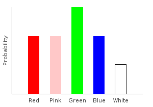
> marblesDist = train bagOfMarbles :: Categorical Double Marble

The Categorical type takes two parameters. The first is the type of our probabilities, and the second is the type of our data points.  If you stick your hand into the bag and draw a random marble, this distribution tells you the probability of drawing each color.

Let’s plot our distribution:

ghci> plotDistribution (plotFile "marblesDist" $ PNG 400 300) marblesDist

Functors

Okay. Now we’re ready for the juicy bits. We’ll start by talking about the list functor.  This will motivate the advantages of the categorical distribution functor.

A functor is a container that lets us “map” a function onto every element of the container.  Lists are a functor, and so we can apply a function to our data set using the map function.

map :: (a -> b) -> [a] -> [b]

Example 1:

Let’s say instead of a distribution over the marbles’ colors, I want a distribution over the marbles’ weights. I might have a function that associates a weight with each type of marble:

> marbleWeight :: Marble -> Int -- weight in grams
> marbleWeight Red   = 3
> marbleWeight Pink  = 2
> marbleWeight Green = 3
> marbleWeight Blue  = 6
> marbleWeight White = 2

I can generate my new distribution by first transforming my data set, and then training on the result.  Notice that the type of our distribution has changed.  It is no longer a categorical distribution over marbles; it’s a distribution over ints.

> weightsDist = train $ map marbleWeight bagOfMarbles :: Categorical Double Int

ghci> plotDistribution (plotFile "weightsDist" $ PNG 400 300) weightsDist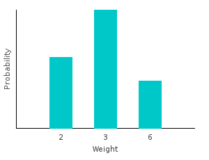

This is the standard way of preprocessing data. But we can do better because the categorical distribution is also a functor. Functors have a function called fmap that is analogous to calling map on a list.  This is its type signature specialized for the Categorical type:

fmap :: (Ord dp0, Ord dp1) => (dp0 -> dp1) -> Categorical prob dp0 -> Categorical prob dp1

We can use fmap to apply the marbleWeights function directly to the distribution:

> weightDist' = fmap marbleWeight marblesDist

This is guaranteed to generate the same exact answer, but it is much faster. It takes only constant time to call Categorical’s fmap, no matter how much data we have!

Let me put that another way. Below is a diagram showing the two possible ways to generate a model on a preprocessed data set.  Every arrow represents a function application.

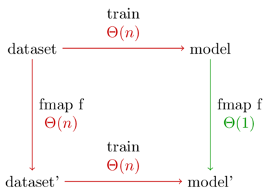
The normal way to preprocess data is to take the bottom left path.  But because our model is a functor, the top right path becomes available.  This path is better because it has the shorter run time.

Furthermore, let’s say we want to experiment with \(latex k\) different preprocessing functions.  The standard method will take \(latex \Theta(nk)\) time, whereas using the categorical functor takes time \(latex \Theta(n + k)\).

Note: The diagram treats the number of different categories (m) as a constant because it doesn’t depend on the number of data points.  In our case, we have 5 types of marbles, so m=5.  Every function call in the diagram is really multiplied by m.

Example 2:

For another example, what if we don’t want to differentiate between red and pink marbles? The following function converts all the pink marbles to red.

> pink2red :: Marble -> Marble 
> pink2red Pink = Red
> pink2red dp   = dp

Let’s apply it to our distribution, and plot the results:

> nopinkDist = fmap pink2red marblesDist

ghci> plotDistribution (plotFile "nopinkDist" $ PNG 400 300) nopinkDist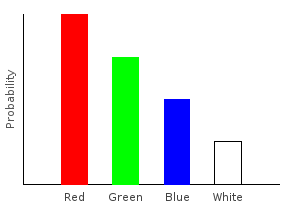

That’s about all that a Functor can do by itself. When we call fmap, we can only process individual data points.  We can’t change the number of points in the resulting distribution or do other complex processing. Monads give us this power.

Monads

Monads are functors with two more functions. The first is called return. Its type signature is

return :: (Ord dp) => dp -> Categorical prob dp

We’ve actually seen this function already in previous posts. It’s equivalent to the train1dp function found in the HomTrainer type class. All it does is train a categorical distribution on a single data point.

The next function is called join. It’s a little bit trickier, and it’s where all the magic lies. Its type signature is:

join :: (Ord dp) => Categorical prob (Categorical prob dp) -> Categorical prob dp

As input, join takes a categorical distribution whose data points are other categorical distributions. It then “flattens” the distribution into one that does not take other distributions as input.

Example 3

Let’s write a function that removes all the pink marbles from our data set.  Whenever we encounter a pink marble, we’ll replace it with an empty categorical distribution; if the marble is not pink, we’ll create a singleton distribution from it.

> forgetPink :: (Num prob) => Marble -> Categorical prob Marble
> forgetPink Pink = mempty
> forgetPink dp   = train1dp dp
>
> nopinkDist2 = join $ fmap forgetPink marblesDist

ghci> plotDistribution (plotFile "nopinkDist2" $ PNG 400 300) nopinkDist2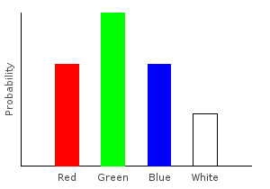

This idiom of join ( fmap … ) is used a lot. For convenience, the** >>=** operator (called bind) combines these steps for us.  It is defined as:

(>>=) :: Categorical prob dp0 -> (dp0 -> Categorical prob dp1) -> Categorical prob dp1
dist >>= f = join $ fmap f dist

Under this notation, our new distribution can be defined as:

> nopinkDist2' = marblesDist >>= forgetPink

Example 4

Besides removing data points, we can also add new ones. Let’s double the number of pink marbles in our training data:

> doublePink :: (Num prob) => Marble -> Categorical prob Marble
> doublePink Pink = 2 .* train1dp Pink
> doublePink dp   = train1dp dp
>
> doublepinkDist = marblesDist >>= doublePink

ghci> plotDistribution (plotFile "doublepinkDist" $ PNG 400 300) doublepinkDist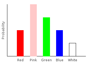

Example 5

Mistakes are often made when collecting data. One common machine learning task is to preprocess data sets to account for these mistakes. In this example, we’ll assume that our sampling process suffers from uniform noise.  Specifically, if one of our data points is red, we will assume there is only a 60% chance that the marble was actually red, and a 10% chance each that it was one of the other colors.  We will define a function to add this noise to our data set, increasing the accuracy of our final distribution.

Notice that we are using fractional weights for our noise, and that the weights are carefully adjusted so that the total number of marbles in the distribution still sums to one.  We don’t want to add or remove marbles while adding noise.

> addNoise :: (Fractional prob) => Marble -> Categorical prob Marble
> addNoise dp = 0.5 .* train1dp dp <> 0.1 .* train [ Red,Pink,Green,Blue,White ]
>
> noiseDist = marblesDist >>= addNoise

ghci> plotDistribution (plotFile "noiseDist" $ PNG 400 300) noiseDist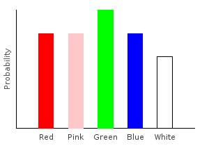

Adding uniform noise just made all our probabilities closer together.

Example 6

Of course, the amount of noise we add to each sample doesn’t have to be the same everywhere. If I suffer from red-green color blindness, then I might use this as my noise function:

> rgNoise :: (Fractional prob) => Marble -> Categorical prob Marble
> rgNoise Red   = trainW [(0.7,Red),(0.3,Green)]
> rgNoise Green = trainW [(0.1,Red),(0.9,Green)]
> rgNoise dp    = train1dp dp 
>
> rgNoiseDist = marblesDist >>= rgNoise

ghci> plotDistribution (plotFile "rgNoiseDist" $ PNG 400 300) rgNoiseDist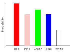

Because of my color blindness, the probability of drawing a red marble from the bag is higher than drawing a green marble.  This is despite the fact that we observed more green marbles in our training data.

Example 7

In the real world, we can never know exactly how much error we have in the samples. Luckily, we can try to learn it by conducting a second experiment. We’ll first experimentally determine how red-green color blind I am, then we’ll use that to update our already trained distribution.

To determine the true error rate, we need some unbiased source of truth. In this case, we can just use someone with good vision. They will select ten red marbles and ten green marbles, and I will guess what color they are.

Let’s train a distribution on what I think green marbles look like:

> greenMarbles = [Green,Red,Green,Red,Green,Red,Red,Green,Green,Green]
> greenDist = train greenMarbles  :: Categorical Double Marble

and what I think red marbles look like:

> redMarbles = [Red,Green,Red,Green,Red,Red,Green,Green,Red,Red]
> redDist = train redMarbles :: Categorical Double Marble

Now we’ll create the noise function based off of our empirical data. The (/.) function is scalar division, and we can use it because the categorical distribution is a vector space. We’re dividing by the number of data points in the distribution so that the distribution we output has an effective training size of one. This ensures that we’re not accidentally creating new data points when applying our function to another distribution.

> rgNoise2 :: Marble -> Categorical Double Marble
> rgNoise2 Green = greenDist /. numdp greenDist
> rgNoise2 Red   = redDist /. numdp redDist
> rgNoise2 dp    = train1dp dp
>
> rgNoiseDist2  = marblesDist >>= rgNoise2

ghci> plotDistribution (plotFile "rgNoiseDist2" $ PNG 400 300) rgNoiseDist2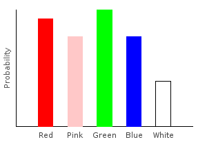

Example 8

We can chain our preprocessing functions together in arbitrary ways.

> allDist = marblesDist >>= forgetPink >>= addNoise >>= rgNoise

ghci> plotDistribution (plotFile "allDist" $ PNG 400 300) allDist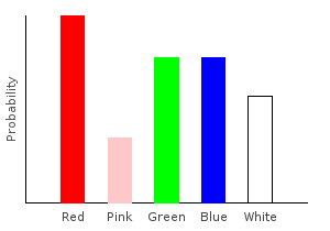

But wait!  Where’d that pink come from?  Wasn’t the call to forgetPink supposed to remove it?  The answer is that we did remove it, but then we added it back in with our noise functions.  When using monadic functions, we must be careful about the order we apply them in.  This is just as true when using regular functions.

Here’s another distribution created from those same functions in a different order:

> allDist2 = marblesDist >>= addNoise >>= rgNoise >>= forgetPink

ghci> plotDistribution (plotFile "allDist" $ PNG 400 300) allDist2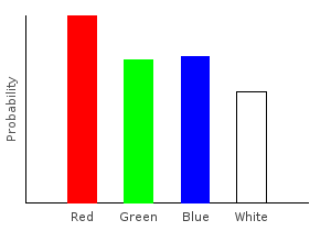

We can also use Haskell’s do notation to accomplish the same exact thing:

>allDist2' :: Categorical Double Marble
>allDist2' = do 
>    dp <- train bagOfMarbles
>    dp <- addNoise dp
>    dp <- rgNoise dp
>    dp <- forgetPink dp
>    return dp

(Since we’re using a custom Monad definition, do notation requires the RebindableSyntax extension.)

Example 9

Do notation gives us a convenient way to preprocess multiple data sets into a single data set. Let’s create two new data sets and their corresponding distributions for us to work with:

> bag1 = [Red,Pink,Green,Blue,White]
> bag2 = [Red,Blue,White]
>
> bag1dist = train bag1 :: Categorical Double Marble
> bag2dist = train bag2 :: Categorical Double Marble

Now, we’ll create a third data set that is a weighted combination of bag1 and bag2. We will do this by repeated sampling. On every iteration, with a 20% probability we’ll sample from bag1, and with an 80% probability we’ll sample from bag2. Imperative pseudo-code for this algorithm is:

let comboDist be an empty distribution
loop until desired accuracy achieved:
    let r be a random number from 0 to 1
    if r > 0.2:
        sample dp1 from bag1
        add dp1 to comboDist
    else:
        sample dp2 from bag2
        add dp2 to comboDist

This sampling procedure will obviously not give us an exact answer. But since the categorical distribution supports weighted data points, we can use this simpler pseudo-code to generate an exact answer:

let comboDist be an empty distribution
foreach datapoint dp1 in bag1:
    foreach datapoint dp2 in bag2:
        add dp1 with weight 0.2 to comboDist
        add dp2 with weight 0.8 to comboDist

Using do notation, we can express this as:

> comboDist :: Categorical Double Marble
> comboDist = do
>   dp1 <- bag1dist
>   dp2 <- bag2dist
>   trainW [(0.2,dp1),(0.8,dp2)]

ghci> plotDistribution (plotFile "comboDist" $ PNG 400 300) comboDist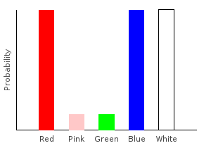

And because the Categorical functor takes constant time, constructing comboDist also takes constant time. The naive imperative algorithm would have taken time \(O(|\text{bag1}|*|\text{bag2}|)\).

When combining multiple distributions this way, the number of data points in our final distribution will be the product of the number of data points in the initial distributions:

ghci> numdp combination
15

Example 10

Finally, arbitrarily complex preprocessing functions can be written using Haskell’s do notation. And remember, no matter how complicated these functions are, their run time never depends on the number of elements in the initial data set.

This function adds uniform sampling noise to our bagOfMarbles, but only on those marbles that are also contained in bag2 above.

> comboDist2 :: Categorical Double Marble
> comboDist2 = do
>   dp1 <- marblesDist
>   dp2 <- bag2dist
>   if dp1==dp2
>       then addNoise dp1
>       else return dp1

ghci> plotDistribution (plotFile "comboDist2" $ PNG 400 300) comboDist2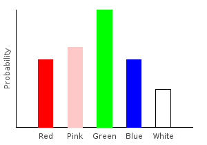

Conclusion

This application of monads to machine learning generalizes the monad used in probabilistic functional programming.  The main difference is that PFP focused on manipulating already known distributions, not training them from data.  Also, if you enjoy this kind of thing, you might be interested in the n-category cafe discussion on category theory in machine learning from a few years back.

In future posts, we’ll look at functors and monads for continuous distributions, multivariate distributions, and classifiers.

Subscribe to the RSS feed to stay tuned!