How to create an unfair coin and prove it with math
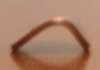
Let’s make some unfair coins by bending them. Our guess is that the concave side will have less area to land on, and so the coin should land on it less often.
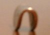
It’s easy to bend the coins with your teeth:
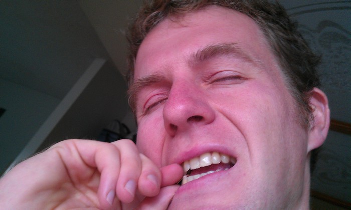
Bending a coin with my teeth
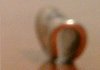
WAIT! That really hurts! Using pliers or wrenches works much better:
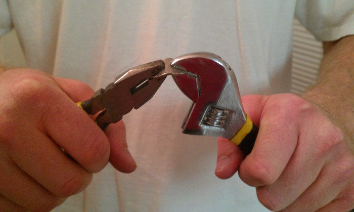
Bending coins with pliers
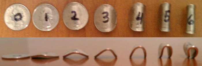
I made seven coins this way, each with a different bending angle.
I did 100 flips for each coin, making sure each flip went at least a foot in the air and spun real well. “Umm… only 100 flips?” you ask, “That can’t be enough!” Just you wait until the section on the math.
Here’s the raw results:
| Coin | Total Flips | Heads | Tails |
| 0 | 100 | 53 | 47 |
| 1 | 100 | 55 | 45 |
| 2 | 100 | 49 | 51 |
| 3 | 100 | 41 | 59 |
| 4 | 100 | 39 | 61 |
| 5 | 100 | 27 | 73 |
| 6 | 100 | 0 | 100 |
Now for the math
Coin flipping is a bernoulli process. This just means that all trials (flips) can have only two outcomes (heads or tails), and each trial is independent of every other trial. What we’re interested in calculating is the expected value of a coin flip for each of our coins. That is, what is the probability it will come up heads? The obvious way to calculate this probability is simply to divide the number of heads by the total number of trials. Unfortunately, this doesn’t give us a good idea about how accurate our estimate is.
Enter the beta distribution. This is a distribution over the bias of a bernoulli process. Intuitively, this means that CDF(x) equals the probability that the expectation of a coin flip is \(\le\) x. In other words, we’re finding the probability that a probability is what we think it should be. That’s a convoluted definition! Some examples should make it clearer.
The beta distribution takes two parameters \(\alpha\) and \(\beta\). \(\alpha\) is the number of heads we have flipped plus one, and \(\beta\) is the number of tails plus one. We’ll talk about why that plus one is there in a bit, but first let’s see what the distribution actually looks like with some example parameters.
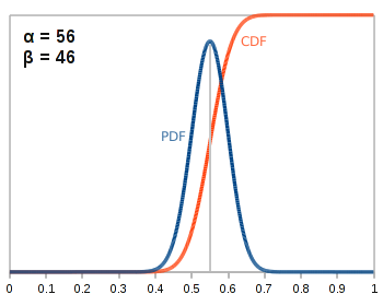
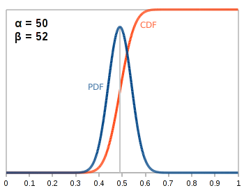
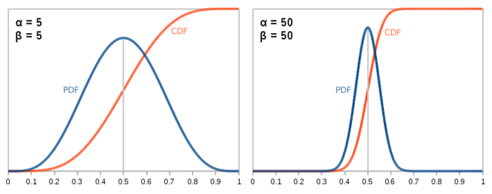 In both the above cases, the distribution is centered around 0.5 because \(\alpha\) and \(\beta\) are equal—we’ve gotten the same number of heads as we have tails. As these parameters increase, the distribution gets tighter and tighter. This should makes sense. The more flips we do, the more confident we can be that the data we’ve collected actually match the characteristics of the coin.
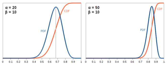
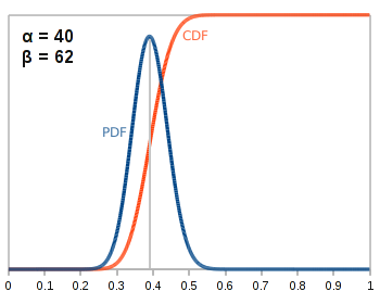
When the parameters are not equal to each other—for example, we’ve seen twice as many heads as we have tails—then the distribution is skewed to the left or right accordingly. The peak of the PDF occurs at:
That’s exactly what we said the expectation of the next coin flip should be above. Awesome!
So what happens when \(\alpha\) and \(\beta\) are one?
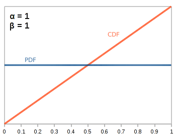
We get the flat distribution. Basically, we haven’t flipped the coin at all yet, so we have no data about how our coin is biased, so all biases are equally likely. This is why we must add one to the number of heads and tails we have flipped to get the appropriate \(\alpha\) and \(\beta\).
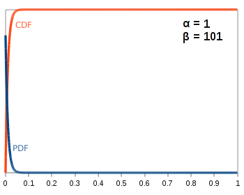
If \(\alpha\) and \(\beta\) are less than one, we get something like this:
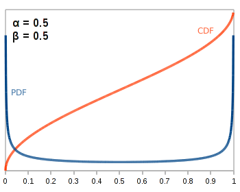
Essentially, this means that we know our coin is very biased in one way or the other, but we don’t know which way yet! As you can imagine, such perverse parameterizations are rarely used in practice.
Hopefully, this has given you an intuitive sense for what the beta distribution looks like. But for the pedantic, here’s how the beta distribution’s pdf is formally defined:
Where \(\Gamma\) is the gamma function—you can think of it as being a generalization of factorials to the real numbers. That is, \(\Gamma(x+1) = (x+1)\Gamma(x) \Leftrightarrow (x+1)! = (x+1) x!\). Excel, many calculators, and any scientific programming package will be able to calculate that for you easily. Most of these applications will even have the beta function already built in.
Applying the beta distribution to our coins
We’re finally ready to see just how biased our coins actually are!
|
Coin 0 
Heads: 53 Tails: 47 |

|
|
Coin 1 Heads: 55 Tails: 45 |
|
|
Coin 2 
Heads: 49 Tails: 51 |
|
|
Coin 3 Heads: 41 Tails: 59 |

|
|
Coin 4 Heads: 39 Tails: 61 |
|
|
Coin 5 Heads: 27 Tails: 73 |

|
|
Coin 6 Heads: 0 Tails: 100 |
|


Amazingly, it takes some pretty big bends to make a biased coin. It’s not until coin 3, which has an almost 90 degree bend that we can say with any confidence that the coin is biased at all. People might notice if you tried to flip that coin to settle a bet!