Markov Networks, Monoids, and Futurama

In this post, we’re going to look at how to manipulate multivariate distributions in Haskell’s HLearn library. There are many ways to represent multivariate distributions, but we’ll use a technique called Markov networks. These networks have the algebraic structure called a monoid (and group and vector space), and training them is a homomorphism. Despite the scary names, these mathematical structures make working with our distributions really easy and convenient—they give us online and parallel training algorithms “for free.” If you want to go into the details of how, you can check out my TFP13 submission, but in this post we’ll ignore those mathy details to focus on how to use the library in practice. We’ll use a running example of creating a distribution over characters in the show Futurama.
Preliminaries: Creating the data Types
As usual, this post is a literate haskell file. To run this code, you’ll need to install the hlearn-distributions package. This package requires GHC version at least 7.6.
bash> cabal install hlearn-distributions-1.1Now for some code. We start with our language extensions and imports:
>{-# LANGUAGE DataKinds #-}
>{-# LANGUAGE TypeFamilies #-}
>{-# LANGUAGE TemplateHaskell #-}
>
>import HLearn.Algebra
>import HLearn.Models.Distributions
Next, we’ll create data type to represent Futurama characters. There are a lot of characters, so we’ll need to keep things pretty organized. The data type will have a record for everything we might want to know about a character. Each of these records will be one of the variables in our multivariate distribution, and all of our data points will have this type.

>data Character = Character
>   { _name      :: String
>   , _species   :: String
>   , _job       :: Job
>   , _isGood    :: Maybe Bool
>   , _age       :: Double -- in years
>   , _height    :: Double -- in feet
>   , _weight    :: Double -- in pounds
>   }
>   deriving (Read,Show,Eq,Ord)
>
>data Job = Manager | Crew | Henchman | Other
>   deriving (Read,Show,Eq,Ord)
Now, in order for our library to be able to interpret the Character type, we call the template haskell function:
>makeTypeLenses ''CharacterThis function creates a bunch of data types and type classes for us. These “type lenses” give us a type-safe way to reference the different variables in our multivariate distribution. We’ll see how to use these type level lenses a bit later. There’s no need to understand what’s going on under the hood, but if you’re curious then checkout the hackage documentation or source code.
Training a distribution
Now, we’re ready to create a data set and start training. Here’s a list of the employees of Planet Express provided by the resident bureaucrat Hermes Conrad. This list will be our first data set.

hermes-zoom
>planetExpress =
>   [ Character "Philip J. Fry"         "human" Crew     (Just True) 1026   5.8 195
>   , Character "Turanga Leela"         "alien" Crew     (Just True) 43     5.9 170
>   , Character "Professor Farnsworth"  "human" Manager  (Just True) 85     5.5 160
>   , Character "Hermes Conrad"         "human" Manager  (Just True) 36     5.3 210
>   , Character "Amy Wong"              "human" Other    (Just True) 21     5.4 140
>   , Character "Zoidberg"              "alien" Other    (Just True) 212    5.8 225
>   , Character "Cubert Farnsworth"     "human" Other    (Just True) 8      4.3 135
>   ]
Let’s train a distribution from this data. Here’s how we would train a distribution where every variable is independent of every other variable:
>dist1 = train planetExpress :: Multivariate Character
>  '[ Independent Categorical '[String,String,Job,Maybe Bool]
>   , Independent Normal '[Double,Double,Double]
>   ]
>   Double
In the HLearn library, we always use the function train to train a model from data points. We specify which model to train in the type signature.
As you can see, the Multivariate distribution takes three type parameters. The first parameter is the type of our data point, in this case Character. The second parameter describes the dependency structure of our distribution. We’ll go over the syntax for the dependency structure in a bit. For now, just notice that it’s a type-level list of distributions. Finally, the third parameter is the type we will use to store our probabilities.
What can we do with this distribution? One simple task we can do is to find marginal distributions. The marginal distribution is the distribution of a certain variable ignoring all the other variables. For example, let’s say I want a distribution of the species that work at planet express. I can get this by:
>dist1a = getMargin TH_species dist1Notice that we specified which variable we’re taking the marginal of by using the type level lens TH_species. This data constructor was automatically created for us by out template haskell function makeTypeLenses. Every one of our records in the data type has its own unique type lens. It’s name is the name of the record, prefixed by TH. These lenses let us infer the types of our marginal distributions at compile time, rather than at run time. For example, the type of the marginal distribution of species is:
ghci> :t dist1a
dist1a :: Categorical String Double
That is, a categorical distributions whose data points are Strings and which stores probabilities as a Double. Now, if I wanted a distribution of the weights of the employees, I can get that by:
>dist1b = getMargin TH_weight dist1And the type of this distribution is:
ghci> :t dist1b
dist1b :: Normal Double
Now, I can easily plot these marginal distributions with the plotDistribution function:
ghci> plotDistribution (plotFile "dist1a" $ PNG 250 250) dist1a
ghci> plotDistribution (plotFile "dist1b" $ PNG 250 250) dist1b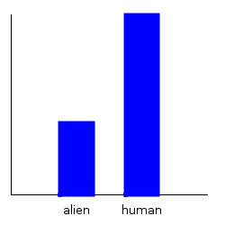


But wait! I accidentally forgot to include Bender in the planetExpress data set! What can I do?
In a traditional statistics library, we would have to retrain our data from scratch. If we had billions of elements in our data set, this would be an expensive mistake. But in our HLearn library, we can take advantage of the model’s monoid structure. In particular, the compiler used this structure to automatically derive a function called add1dp for us. Let’s look at its type:
ghci> :t add1dp
add1dp :: HomTrainer model => model -> Datapoint model -> model
It’s pretty simple. The function takes a model and adds the data point associated with that model. It returns the model we would have gotten if the data point had been in our original data set. This is called online training.
Again, because our distributions form monoids, the compiler derived an efficient and exact online training algorithm for us automatically.
So let’s create a new distribution that considers bender:
>bender = Character "Bender Rodriguez" "robot" Crew (Just True) 44 6.1 612
>dist1' = add1dp dist1 bender
And plot our new marginals:
ghci> plotDistribution (plotFile "dist1-withbender-species" $ PNG 250 250) $
                getMargin TH_species dist1'
ghci> plotDistribution (plotFile "dist1-withbender-weight"  $ PNG 250 250) $
                getMargin TH_weight dist1'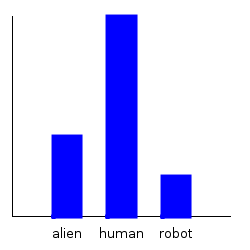

Notice that our categorical marginal has clearly changed, but that our normal marginal doesn’t seemed to have changed at all. This is because the plotting routines automatically scale the distribution, and the normal distribution, when scaled, always looks the same. We can double check that we actually did change the weight distribution by comparing the mean:
ghci> mean dist1b
176.42857142857142
ghci> mean $ getMargin TH_weight dist1'
230.875
Bender’s weight really changed the distribution after all!
Complicated DependencE structureS
That’s cool, but our original distribution isn’t very interesting. What makes multivariate distributions interesting is when the variables affect each other. This is true in our case, so we’d like to be able to model it. For example, we’ve already seen that robots are much heavier than organic lifeforms, and are throwing off our statistics. The HLearn library supports a small subset of Markov Networks for expressing these dependencies.
We represent Markov Networks as graphs with undirected edges. Every attribute in our distribution is a node, and every dependence between attributes is an edge. We can draw this graph with the plotNetwork command:
ghci> plotNetwork "dist1-network" dist1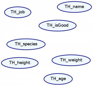
As expected, there are no edges in our graph because everything is independent. Let’s create a more interesting distribution and plot its Markov network.
    >dist2 = train planetExpress :: Multivariate Character
    >  '[ Ignore                  '[String]
    >   , MultiCategorical        '[String]
    >   , Independent Categorical '[Job,Maybe Bool]
    >   , Independent Normal      '[Double,Double,Double]
    >   ]
    >   Double
ghci> plotNetwork "dist2-network" dist2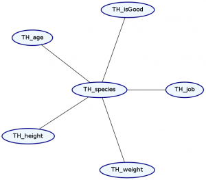
Okay, so what just happened?
The syntax for representing the dependence structure is a little confusing, so let’s go step by step. We represent the dependence information in the graph as a list of types. Each element in the list describes both the marginal distribution and the dependence structure for one or more records in our data type. We must list these elements in the same order as the original data type.
Notice that we’ve made two changes to the list. First, our list now starts with the type Ignore ’[String]. This means that the first string in our data type—the name—will be ignored. Notice that TH_name is no longer in the Markov Network. This makes sense because we expect that a character’s name should not tell us too much about any of their other attributes.
Second, we’ve added a dependence. The MultiCategorical distribution makes everything afterward in the list dependent on that item, but not the things before it. This means that the exact types of dependencies it can specify are dependent on the order of the records in our data type. Let’s see what happens if we change the location of the MultiCategorical:
    >dist3 = train planetExpress :: Multivariate Character
    >  '[ Ignore '[String]
    >   , Independent Categorical '[String]
    >   , MultiCategorical '[Job]
    >   , Independent Categorical '[Maybe Bool]
    >   , Independent Normal '[Double,Double,Double]
    >   ]
    >   Double
ghci> plotNetwork "dist3-network" dist3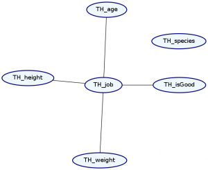
As you can see, our species no longer have any relation to anything else. Unfortunately, using this syntax, the order of list elements is important, and so the order we specify our data records is important.
Finally, we can substitute any valid univariate distribution for our Normal and Categorical distributions. The HLearn library currently supports Binomial, Exponential, Geometric, LogNormal, and Poisson distributions. These just don’t make much sense for modelling Futurama characters, so we’re not using them.
Now, we might be tempted to specify that every variable is fully dependent on every other variable. In order to do this, we have to introduce the “Dependent” type. Any valid multivariate distribution can follow Dependent, but only those records specified in the type-list will actually be dependent on each other. For example:
    >dist4 = train planetExpress :: Multivariate Character
    >  '[ Ignore '[String]
    >   , MultiCategorical '[String,Job,Maybe Bool]
    >   , Dependent MultiNormal '[Double,Double,Double]
    >   ]
    >   Double
ghci> plotNetwork "dist4-network" dist4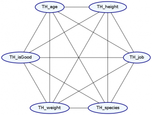
Undoubtably, this is in always going to be the case—everything always has a slight influence on everything else. Unfortunately, it is not easy in practice to model these fully dependent distributions. We need roughly \(\Theta(2^{n+e})\) data points to accurately train a distribution, where n is the number of nodes in our graph and e is the number of edges in our network. Thus, by selecting that two attributes are independent of each other, we can greatly reduce the amount of data we need to train an accurate distribution.
I realize that this syntax is a little awkward. I chose it because it was relatively easy to implement. Future versions of the library should support a more intuitive syntax. I also plan to use copulas to greatly expand the expressiveness of these distributions. In the mean time, the best way to figure out the dependencies in a Markov Network are just to plot it and see visually.
Okay. So what distribution makes the most sense for Futurama characters? We’ll say that everything depends on both the characters’ species and job, and that their weight depends on their height.
    >planetExpressDist = train planetExpress :: Multivariate Character
    >  '[ Ignore '[String]
    >   , MultiCategorical '[String,Job]
    >   , Independent Categorical '[Maybe Bool]
    >   , Independent Normal '[Double]
    >   , Dependent MultiNormal '[Double,Double]
    >   ]
    >   Double
ghci> plotNetwork "planetExpress-network" planetExpressDist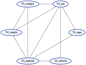
We still don’t have enough data to to train this network, so let’s create some more. We start by creating a type for our Markov network called FuturamaDist. This is just for convenience so we don’t have to retype the dependence structure many times.
>type FuturamaDist = Multivariate Character
>  '[ Ignore '[String]
>   , MultiCategorical '[String,Job]
>   , Independent Categorical '[Maybe Bool]
>   , Independent Normal '[Double]
>   , Dependent MultiNormal '[Double,Double]
>   ]
>   Double
Next, we train some more distribubtions of this type on some of the characters. We’ll start with Mom Corporation and the brave Space Forces.


    >momCorporation =
    >   [ Character "Mom"                   "human" Manager  (Just False) 100 5.5 130
    >   , Character "Walt"                  "human" Henchman (Just False) 22  6.1 170
    >   , Character "Larry"                 "human" Henchman (Just False) 18  5.9 180
    >   , Character "Igner"                 "human" Henchman (Just False) 15  5.8 175
    >   ]
    >momDist = train momCorporation :: FuturamaDist
>spaceForce =
> [ Character "Zapp Brannigan" "human" Manager (Nothing) 45 6.0 230
> , Character "Kif Kroker" "alien" Crew (Just True) 113 4.5 120
> ]
>spaceDist = train spaceForce :: FuturamaDistAnd now some more robots:


>robots =
>   [ bender
>   , Character "Calculon"              "robot" Other    (Nothing)    123  6.8 650
>   , Character "The Crushinator"       "robot" Other    (Nothing)    45   8.0 4500
>   , Character "Clamps"                "robot" Henchman (Just False) 134  5.8 330
>   , Character "DonBot"                "robot" Manager  (Just False) 178  5.8 520
>   , Character "Hedonismbot"           "robot" Other    (Just False) 69   4.3 1200
>   , Character "Preacherbot"           "robot" Manager  (Nothing)    45   5.8 350
>   , Character "Roberto"               "robot" Other    (Just False) 77   5.9 250
>   , Character "Robot Devil"           "robot" Other    (Just False) 895  6.0 280
>   , Character "Robot Santa"           "robot" Other    (Just False) 488  6.3 950
>   ]
>robotDist = train robots :: FuturamaDist
Now we’re going to take advantage of the monoid structure of our multivariate distributions to combine all of these distributions into one.
> futuramaDist = planetExpressDist <> momDist <> spaceDist <> robotDistThe resulting distribution is equivalent to having trained a distribution from scratch on all of the data points:
train (planetExpress++momCorporation++spaceForces++robots) :: FuturamaDistWe can take advantage of this property any time we use the train function to automatically parallelize our code. The higher order function parallel will split the training task evenly over each of your available processors, then merge them together with the monoid operation. This results in “theoretically perfect” parallel training of these models.
parallel train (planetExpress++momCorporation++spaceForces++robots) :: FuturamaDistAgain, this is only possible because the distributions have a monoid structure.
Now, let’s ask some questions of our distribution. If I pick a character at random, what’s the probability that they’re a good guy? Let’s plot the marginal.
ghci> plotDistribution (plotFile "goodguy" $ PNG 250 250) $ getMargin TH_isGood futuramaDist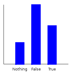
But what if I only want to pick from those characters that are humans, or those characters that are robots? Statisticians call this conditioning. We can do that with the condition function:
ghci> plotDistribution (plotFile "goodguy-human" $ PNG 250 250) $
             getMargin TH_isGood $ condition TH_species "human" futuramaDist
ghci> plotDistribution (plotFile "goodguy-robot" $ PNG 250 250) $
             getMargin TH_isGood $ condition TH_species "robot" futuramaDist

On the left is the plot for humans, and on the right the plot for robots. Apparently, original robot sin is much worse than that in humans! If only they would listen to Preacherbot and repent of their wicked ways…
Now let’s ask: What’s the average age of an evil robot?
ghci> mean $ getMargin TH_age $
         condition TH_isGood (Just False) $ condition TH_species "robot" futuramaDist
273.0769230769231
Notice that conditioning a distribution is a commutative operation. That means we can condition in any order and still get the exact same results. Let’s try it:
ghci> mean $ getMargin TH_age $
         condition TH_species "robot" $ condition TH_isGood (Just False) futuramaDist
273.0769230769231
There’s one last thing for us to consider. What does our Markov network look like after conditioning? Let’s find out!
plotNetwork "condition-species-isGood" $
         condition TH_species "robot" $ condition TH_isGood (Just False) futuramaDist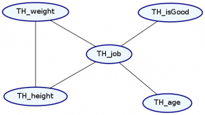
Notice that conditioning against these variables caused them to go away from our Markov Network.
Finally, there’s another similar process to conditioning called “marginalizing out.” This lets us ignore the effects of a single attribute without specifically saying what that attribute must be. When we marginalize out on our Markov network, we get the same dependence structure as if we conditioned.
plotNetwork "marginalizeOut-species-isGood" $
         marginalizeOut TH_species $ marginalizeOut TH_isGood futuramaDist
Effectively, what the marginalizeOut function does is “forget” the extra dependencies, whereas the condition function “applies” those dependencies. In the end, the resulting Markov network has the same structure, but different values.
Finally, at the start of the post, I mentioned that our multivariate distributions have group and vector space structure. This gives us two more operations we can use: the inverse and scalar multiplication. You can find more posts on how to take advantage of these structures here and here.
Next time…

The best part of all of this is still coming. Next, we’ll take a look at full on Bayesian classification and why it forms a monoid. Besides online and parallel trainers, this also gives us a fast cross-validation method.
There’ll also be a posts about the monoid structure of Markov chains, the Free HomTrainer, and how this whole algebraic framework applies to NP-approximation algorithms as well.