Nuclear weapon statistics using monoids, groups, and modules in Haskell
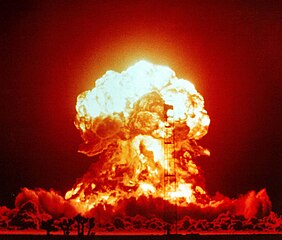
The Bulletin of the Atomic Scientists tracks the nuclear capabilities of every country. We’re going to use their data to demonstrate Haskell’s HLearn library and the usefulness of abstract algebra to statistics. Specifically, we’ll see that the categorical distribution and kernel density estimates have monoid, group, and module algebraic structures. We’ll explain what this crazy lingo even means, then take advantage of these structures to efficiently answer real-world statistical questions about nuclear war. It’ll be a WOPR!
Before we get into the math, we’ll need to review the basics of nuclear politics.
The nuclear Non-Proliferation Treaty (NPT) is the main treaty governing nuclear weapons. Basically, it says that there are five countries that are “allowed” to have nukes: the USA, UK, France, Russia, and China. “Allowed” is in quotes because the treaty specifies that these countries must eventually get rid of their nuclear weapons at some future, unspecified date. When another country, for example Iran, signs the NPT, they are agreeing to not develop nuclear weapons. What they get in exchange is help from the 5 nuclear weapons states in developing their own civilian nuclear power programs. (Iran has the legitimate complaint that Western countries are actively trying to stop its civilian nuclear program when they’re supposed to be helping it, but that’s a whole ’nother can of worms.)
The Nuclear Notebook tracks the nuclear capabilities of all these countries. The most-current estimates are from mid-2012. Here’s a summary (click the warhead type for more info):| Country | Delivery Method | Warhead | Yield (kt) | # Deployed |
| USA | ICBM | W78 | 335 | 250 |
| USA | ICBM | W87 | 300 | 250 |
| USA | SLBM | W76 | 100 | 468 |
| USA | SLBM | W76-1 | 100 | 300 |
| USA | SLBM | W88 | 455 | 384 |
| USA | Bomber | W80 | 150 | 200 |
| USA | Bomber | B61 | 340 | 50 |
| USA | Bomber | B83 | 1200 | 50 |
| UK | SLBM | W76 | 100 | 225 |
| France | SLBM | TN75 | 100 | 150 |
| France | Bomber | TN81 | 300 | 150 |
| Russia | ICBM | RS-20V | 800 | 500 |
| Russia | ICBM | RS-18 | 400 | 288 |
| Russia | ICBM | RS-12M | 800 | 135 |
| Russia | ICBM | RS-12M2 | 800 | 56 |
| Russia | ICBM | RS-12M1 | 800 | 18 |
| Russia | ICBM | RS-24 | 100 | 90 |
| Russia | SLBM | RSM-50 | 50 | 144 |
| Russia | SLBM | RSM-54 | 100 | 384 |
| Russia | Bomber | AS-15 | 200 | 820 |
| China | ICBM | DF-3A | 3300 | 16 |
| China | ICBM | DF-4 | 3300 | 12 |
| China | ICBM | DF-5A | 5000 | 20 |
| China | ICBM | DF-21 | 300 | 60 |
| China | ICBM | DF-31 | 300 | 20 |
| China | ICBM | DF-31A | 300 | 20 |
| China | Bomber | H-6 | 3100 | 20 |
I’ve consolidated all this data into the file nukes-list.csv, which we will analyze in this post. If you want to try out this code for yourself (or the homework question at the end), you’ll need to download it. Every line in the file corresponds to a single nuclear warhead, not delivery method. Warheads are the parts that go boom! Bombers, ICBMs, and SSBN/SLBMs are the delivery method.

nuclear-triad
There are three things to note about this data. First, it’s only estimates based on public sources. In particular, it probably overestimates the Russian nuclear forces. Other estimates are considerably lower. Second, we will only be considering deployed, strategic warheads. Basically, this means the “really big nukes that are currently aimed at another country.” There are thousands more tactical warheads, and warheads in reserve stockpiles waiting to be disassembled. For simplicity—and because these nukes don’t significantly affect strategic planning—we won’t be considering them here. Finally, there are 4 countries who are not members of the NPT but have nuclear weapons: Israel, Pakistan, India, and North Korea. We will be ignoring them here because their inventories are relatively small, and most of their weapons would not be considered strategic.
Programming preliminaries
First, let’s install the library:
$ cabal install HLearn-distributions-0.1Now we’re ready to start programming. First, let’s import our libraries:
>import Control.Lens
>import Data.Csv
>import qualified Data.Vector as V
>import qualified Data.ByteString.Lazy.Char8  as BS
>
>import HLearn.Algebra
>import HLearn.Models.Distributions
>import HLearn.Gnuplot.Distributions
Next, we load our data using the Cassava package. (You don’t need to understand how this works.)
>main = do
>    Right rawdata <- fmap (fmap V.toList . decode True) $ BS.readFile "nukes-list.csv"
>        :: IO (Either String [(String, String, String, Int)])
And we’ll use the Lens package to parse the CSV file into a series of variables containing just the values we want. (You also don’t need to understand this.)
>   let list_usa    = fmap (\row -> row^._4) $ filter (\row -> (row^._1)=="USA"   ) rawdata
>   let list_uk     = fmap (\row -> row^._4) $ filter (\row -> (row^._1)=="UK"    ) rawdata
>   let list_france = fmap (\row -> row^._4) $ filter (\row -> (row^._1)=="France") rawdata
>   let list_russia = fmap (\row -> row^._4) $ filter (\row -> (row^._1)=="Russia") rawdata
>   let list_china  = fmap (\row -> row^._4) $ filter (\row -> (row^._1)=="China" ) rawdata
NOTE: All you need to understand about the above code is what these list_country variables look like. So let’s print one:
> putStrLn $ "List of American nuclear weapon sizes = " ++ show list_usagives us the output:
List of American nuclear weapon sizes = fromList [335,335,335,335,335,335,335,335,335,335 ... 1200,1200,1200,1200,1200]If we want to know how many weapons are in the American arsenal, we can take the length of the list:
> putStrLn $ "Number of American weapons = " ++ show (length list_usa)We get that there are 1951 American deployed, strategic nuclear weapons. If we want to know the total “blowing up” power, we take the sum of the list:
> putStrLn $ "Explosive power of American weapons = " ++ show (sum list_usa)We get that the US has 516 megatons of deployed, strategic nuclear weapons. That’s the equivalent of 1,033,870,000,000 pounds of TNT.
To get the total number of weapons in the world, we concatenate every country’s list of weapons and find the length:
>   let list_all = list_usa ++ list_uk ++ list_france ++ list_russia ++ list_china
> putStrLn $ "Number of nukes in the whole world = " ++ show (length list_all)| Country | Warheads | Total explosive power (kt) |
| USA | 1,951 | 516,935 |
| UK | 225 | 22,500 |
| France | 300 | 60,000 |
| Russia | 2,435 | 901,000 |
| China | 168 | 284,400 |
| Total | 5,079 | 1,784,835 |
Now let’s do some algebra!
Monoids and groups
In a previous post, we saw that the Gaussian distribution forms a group. This means that it has all the properties of a monoid—an empty element (mempty) that represents the distribution trained on no data, and a binary operation (mappend) that merges two distributions together—plus an inverse. This inverse lets us “subtract” two Gaussians from each other.
It turns out that many other distributions also have this group property. For example, the categorical distribution. This distribution is used for measuring discrete data. Essentially, it assigns some probability to each “label.” In our case, the labels are the size of the nuclear weapon, and the probability is the chance that a randomly chosen nuke will be exactly that destructive. We train our categorical distribution using the train function:
> let cat_usa = train list_usa :: Categorical Int DoubleIf we plot this distribution, we’ll get a graph that looks something like:
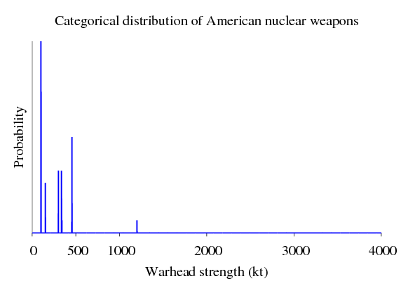
A distribution like this is useful to war planners from other countries. It can help them statistically determine the amount of casualties their infrastructure will take from a nuclear exchange.
Now, let’s train equivalent distributions for our other countries.
> let cat_uk = train list_uk :: Categorical Int Double
> let cat_france = train list_france :: Categorical Int Double
> let cat_russia = train list_russia :: Categorical Int Double
> let cat_china = train list_china :: Categorical Int Double
Because training the categorical distribution is a group homomorphism, we can train a distribution over all nukes by either training directly on the data:
> let cat_allA = train list_all :: Categorical Int Doubleor we can merge the already generated categorical distributions:
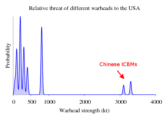
> let cat_allB = cat_usa <> cat_uk <> cat_france <> cat_russia <> cat_chinaBecause of the homomorphism property, we will get the same result both ways. Since we’ve already done the calculations for each of the the countries already, method B will be more efficient—it won’t have to repeat work we’ve already done. If we plot either of these distributions, we get:
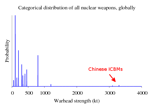
The thing to notice in this plot is that most countries have a nuclear arsenal that is distributed similarly to the United States—except for China. These Chinese ICBMs will become much more important when we discuss nuclear strategy in the last section.
But nuclear war planners don’t particularly care about this complete list of nuclear weapons. What war planners care about is the survivable nuclear weapons—that is, weapons that won’t be blown up by a surprise nuclear attack. Our distributions above contain nukes dropped from bombers, but these are not survivable. They are easy to destroy. For our purposes, we’ll call anything that’s not a bomber a survivable weapon.

nuclear-triad-no-bomber
We’ll use the group property of the categorical distribution to calculate the survivable weapons. First, we create a distribution of just the _un_survivable bombers:
>   let list_bomber = fmap (\row -> row^._4) $ filter (\row -> (row^._2)=="Bomber") rawdata
>   let cat_bomber = train list_bomber :: Categorical Int Double
Then, we use our group inverse to subtract these unsurvivable weapons away:
> let cat_survivable = cat_allB <> (inverse cat_bomber)Notice that we calculated this distribution indirectly—there was no possible way to combine our variables above to generate this value without using the inverse! This is the power of groups in statistics.
More distributions
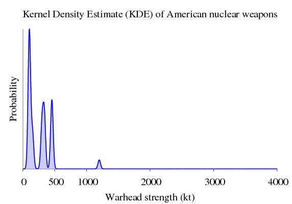
The categorical distribution is not sufficient to accurately describe the distribution of nuclear weapons. This is because we don’t actually know the yield of a given warhead. Like all things, it has some manufacturing tolerances that we must consider. For example, if we detonate a 300 kt warhead, the actual explosion might be 275 kt, 350 kt, or the bomb might even “fizzle out” and have almost a 0kt explosion.
We’ll model this by using a kernel density estimator (KDE). The KDE basically takes all our data points, assigns each one a probability distribution called a “kernel,” then sums these kernels together. It is a very powerful and general technique for modelling distributions… and it also happens to form a group!
First, let’s create the parameters for our KDE. The bandwidth controls how wide each of the kernels is. Bigger means wider. I selected 20 because it made a reasonable looking density function. The sample points are exactly what they sounds like: they are where we will sample the density from. We can generate them using the function genSamplePoints. Finally, the kernel is the shape of the distributions we will be summing up. There are many supported kernels.
>   let kdeparams = KDEParams
>        { bandwidth    = Constant 20
>        , samplePoints = genSamplePoints
>               0       -- minimum
>               4000    -- maximum
>               4000    -- number of samples
>        , kernel       = KernelBox Gaussian
>        } :: KDEParams Double
Now, we’ll train kernel density estimates on our data. Notice that because the KDE takes parameters, we must use the train’ function instead of just train.
> let kde_usa = train' kdeparams list_usa :: KDE DoubleAgain, plotting just the American weapons gives:
kernel density estimate of american nuclear weapons
And we train the corresponding distributions for the other countries.
>   let kde_uk      = train' kdeparams list_uk       :: KDE Double
>   let kde_france  = train' kdeparams list_france   :: KDE Double
>   let kde_russia  = train' kdeparams list_russia   :: KDE Double
>   let kde_china   = train' kdeparams list_china    :: KDE Double
>
>   let kde_all = kde_usa <> kde_uk <> kde_france <> kde_russia <> kde_china
The KDE is a powerful technique, but the draw back is that it is computationally expensive—especially when a large number of sample points are used. Fortunately, all computations in the HLearn library are easily parallelizable by applying the higher order function parallel.
We can calculate the full KDE from scratch in parallel like this:
>   let list_double_all = map fromIntegral list_all :: [Double]
>   let kde_all_parA = (parallel (train' kdeparams)) list_double_all :: KDE Double
or we can perform a parallel reduction on the KDEs for each country like this:
> let kde_all_parB = (parallel reduce) [kde_usa, kde_uk, kde_france, kde_russia, kde_china]And because the KDE is a homomorphism, we get the same exact thing either way. Let’s plot the parallel version:
> plotDistribution (genPlotParams "kde_all" kde_all_parA) kde_all_parA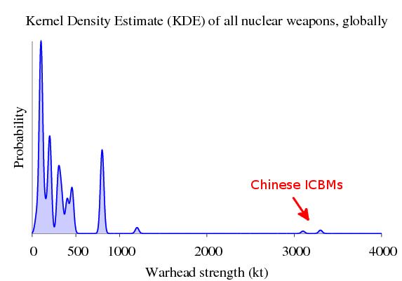
The parallel computation takes about 16 seconds on my Core2 Duo laptop running on 2 processors, whereas the serial computation takes about 28 seconds.
This is a considerable speedup, but we can still do better. It turns out that there is a homomorphism from the Categorical distribution to the KDE:
>   let kde_fromcat_all = cat_allB $> kdeparams
>   plotDistribution (genPlotParams "kde_fromcat_all" kde_fromcat_all) kde_fromcat_all
(For more information about the morphism chaining operator $>, see the Hlearn documentation.) This computation takes less than a second and gets the exact same result as the much more expensive computations above.
We can express this relationship with a commutative diagram:
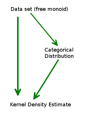
No matter which path we take to get to a KDE, we will get the exact same answer. So we should always take the path that will be least computationally expensive for the data set we’re working on.
Why does this work? Well, the categorical distribution is a structure called the “free module” in disguise.
Modules and the Free Module
R-Modules (like groups, but unlike monoids) have not seen much love from functional programmers. This is a shame, because they’re quite handy. It turns out they will increase our performance dramatically in this case.
It’s not super important to know the formal definition of an R-module, but here it is anyways: An R-module is a group with an additional property: it can be “multiplied” by any element of the ring R. This is a generalization of vector spaces because R need only be a ring instead of a field. (Rings do not necessarily have multiplicative inverses.) It’s probably easier to see what this means by an example.
Vectors are modules. Let’s say I have a vector:
> let vec = [1,2,3,4,5] :: [Int]I can perform scalar multiplication on that vector like this:
> let vec2 = 3 .* vecwhich as you might expect results in:
[3,6,9,12,15]Our next example is the free R-module. A “free” structure is one that obeys only the axioms of the structure and nothing else. Functional programmers are very familiar with the free monoid—it’s the list data type. The free Z-module is like a beefed up list. Instead of just storing the elements in a list, it also stores the number of times that element occurred. (Z is shorthand for the set of integers, which form a ring but not a field.) This lets us greatly reduce the memory required to store a repetitive data set.
In HLearn, we represent the free module over a ring r with the data type:
:: FreeMod r awhere a is the type of elements to be stored in the free module. We can convert our lists into free modules using the function list2module like this:
> let module_usa = list2module list_usaBut what does the free module actually look like? Let’s print it to find out:
> print module_usagives us:
FreeMod (fromList [(100,768),(150,200),(300,250),(335,249),(340,50),(455,384),(1200,50)])This is much more compact! So this is the take away: The free module makes repetitive data sets easier to work with. Now, let’s convert all our country data into module form:
>   let module_uk       = list2module list_uk
>   let module_france   = list2module list_france
>   let module_russia   = list2module list_russia
>   let module_china    = list2module list_china
Because modules are also groups, we can combine them like so:
> let module_allA = module_usa <> module_uk <> module_france <> module_russia <> module_chinaor, we could train them from scratch:
> let module_allB = list2module list_allAgain, because generating a free module is a homomorphism, both methods are equivalent.
Module distributions
The categorical distribution and the KDE both have this module structure. This gives us two cool properties for free.
First, we can train these distributions directly from the free module. Because the free module is potentially much more compact than a list is, this can save both memory and time. If we run:
>   let cat_module_all = train module_allB :: Categorical Int Double
>   let kde_module_all = train' kdeparams module_allB :: KDE Double
Then we get the properties:
cat_mod_all == cat_all
kde_mod_all == kde_all == kde_cat_all
Extending our commutative diagram above gives:
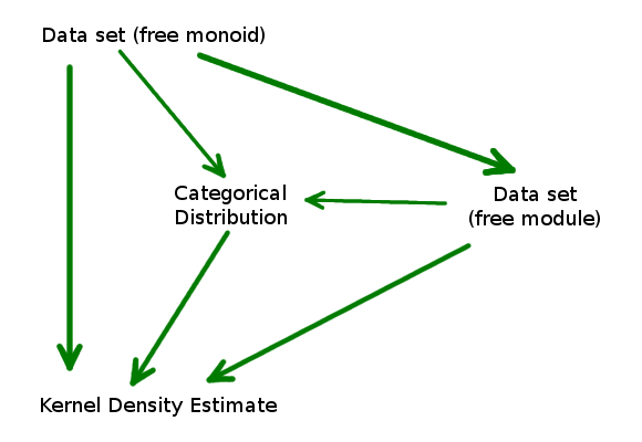
Again, no matter which path we take to train our KDE, we still get the same result because each of these arrows is a homomorphism.
Second, if a distribution is a module, we can weight the importance of our data points. Let’s say we’re a general from North Korea (DPRK), and we’re planning our nuclear strategy. The US and North Korea have a very strained relationship in the nuclear department. It is much more likely that the US will try to nuke the DPRK than China will. And modules let us model this! We can weight each country’s influence on our “nuclear threat profile” distribution like this:
>   let threats_dprk = 20 .* kde_usa
>                   <> 10 .* kde_uk
>                   <> 5  .* kde_france
>                   <> 2  .* kde_russia
>                   <> 1  .* kde_china
>
>   plotDistribution (genPlotParams "threats_dprk" threats_dprk) threats_dprk
Basically, we’re saying that the USA is 20x more likely to attack the DPRK than China is. Graphically, our threat distribution is:
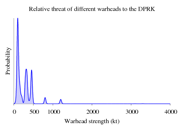
The maximum threat that we have to worry about is about 1300 kt, so we need to design all our nuclear bunkers to withstand this level of blast. Nuclear war planners would use the above distribution to figure out how much infrastructure would survive a nuclear exchange. To see how this is done, you’ll have to click the link.
On the other hand, if we’re an American general, then we might say that China is our biggest threat… who knows what they’ll do when we can’t pay all the debt we owe them!?
>   let threats_usa = 1 .* kde_russia
>                  <> 5 .* kde_china
>
>   plotDistribution (genPlotParams "threats_usa" threats_usa) threats_usa
Graphically:
So now Chinese ICBMs are a real threat. For American infrastructure to be secure, most of it needs to be able to withstand ~3500 kt blast. (Actually, Chinese nuclear policy is called the “minimum means of reprisal”—these nukes are not targeted at military installations, but major cities. Unlike the other nuclear powers, China doesn’t hope to win a nuclear war. Instead, its nuclear posture is designed to prevent nuclear war in the first place. This is why China has the fewest weapons of any of these countries. For a detailed analysis, see the book Minimum Means of Reprisal. This means that American military infrastructure isn’t threatened by these large Chinese nukes, and really only needs to be able to withstand an 800kt explosion to be survivable.)
By the way, since we’ve already calculated all of the kde_country variables before, these computations take virtually no time at all to compute. Again, this is all made possible thanks to our friend abstract algebra.
Homework + next Post
If you want to try out the HLearn library for yourself, here’s a question you can try to answer: Create the DPRK and US threat distributions above, but only use survivable weapons. Don’t include bombers in the analysis.
In our next post, we’ll go into more detail about the mathematical plumbing that makes all this possible. Then we’ll start talking about Bayesian classification and full-on machine learning. Subscribe to the RSS feed so you don’t miss out!
Why don’t you listen to Tom Lehrer’s “Song for WWIII” while you wait?