Gausian distributions form a monoid

(And why machine learning experts should care)

This is the first in a series of posts about the HLearn library for haskell that I’ve been working on for the past few months. The idea of the library is to show that abstract algebra—specifically monoids, groups, and homomorphisms—are useful not just in esoteric functional programming, but also in real world machine learning problems.  In particular, by framing a learning algorithm according to these algebraic properties, we get three things for free: (1) an online version of the algorithm; (2) a parallel version of the algorithm; and (3) a procedure for cross-validation that runs asymptotically faster than the standard version.

We’ll start with the example of a Gaussian distribution. Gaussians are ubiquitous in learning algorithms because they accurately describe most data.  But more importantly, they are easy to work with.  They are fully determined by their mean and variance, and these parameters are easy to calculate.

In this post we’ll start with examples of why the monoid and group properties of Gaussians are useful in practice, then we’ll look at the math underlying these examples, and finally we’ll see that this technique is extremely fast in practice and results in near perfect parallelization.

HLearn by Example

Install the libraries from a shell:

$ cabal install HLearn-distributions

Then import the HLearn libraries into a literate haskell file:

> import HLearn.Algebra
> import HLearn.Models.Distributions.Gaussian

And some libraries for comparing our performance:

> import Criterion.Main
> import Statistics.Distribution.Normal
> import qualified Data.Vector.Unboxed as VU

Now let’s create some data to work with. For simplicity’s sake, we’ll use a made up data set of how much money people make. Every entry represents one person making that salary. (We use a small data set here for ease of explanation.  When we stress test this library at the end of the post we use much larger data sets.)

> gradstudents = [15e3,25e3,18e3,17e3,9e3]        :: [Double]
> teachers     = [40e3,35e3,89e3,50e3,52e3,97e3]  :: [Double]
> doctors      = [130e3,105e3,250e3]              :: [Double]

In order to train a Gaussian distribution from the data, we simply use the train function, like so:

> gradstudents_gaussian = train gradstudents      :: Gaussian Double
> teachers_gaussian     = train teachers          :: Gaussian Double
> doctors_gaussian      = train doctors           :: Gaussian Double

The train function is a member of the HomTrainer type class, which we’ll talk more about later.  Also, now that we’ve trained some Gaussian distributions, we can perform all the normal calculations we might want to do on a distribution.  For example, taking the mean, standard deviation, pdf, and cdf.

Now for the interesting bits. We start by showing that the Gaussian is a semigroup. A semigroup is any data structure that has an associative binary operation called (<>). Basically, we can think of (<>) as “adding” or “merging” the two structures together. (Semigroups are monoids with only a mappend function.)

So how do we use this? Well, what if we decide we want a Gaussian over everyone’s salaries? Using the traditional approach, we’d have to recompute this from scratch.

> all_salaries = concat [gradstudents,teachers,doctors]
> traditional_all_gaussian = train all_salaries :: Gaussian Double

But this repeats work we’ve already done. On a real world data set with millions or billions of samples, this would be very slow. Better would be to merge the Gaussians we’ve already trained into one final Gaussian. We can do that with the semigroup operation (<>):

> semigroup_all_gaussian = gradstudents_gaussian <> teachers_gaussian <> doctors_gaussian

Now,

traditional_all_gaussian == semigroup_all_gaussian

The coolest part about this is that the semigroup operation takes time O(1), no matter how much data we’ve trained the Gaussians on. The naive approach takes time O(n), so we’ve got a pretty big speed up!

Next, a monoid is a semigroup with an identity. The identity for a Gaussian is easy to define—simply train on the empty data set!

> gaussian_identity = train ([]::[Double]) :: Gaussian Double

Now,

gaussian_identity == mempty

But we’ve still got one more trick up our sleeves.  The Gaussian distribution is not just a monoid, but also a group. Groups appear all the time in abstract algebra, but they haven’t seen much attention in functional programming for some reason. Well groups are simple: they’re just monoids with an inverse. This inverse lets us do “subtraction” on our data structures.

So back to our salary example. Lets say we’ve calculated all our salaries, but we’ve realized that including grad students in the salary calculations was a mistake. (They’re not real people after all.) In a normal library, we would have to recalculate everything from scratch again, excluding the grad students:

> nograds = concat [teachers,doctors]
> traditional_nograds_gaussian = train nograds :: Gaussian Double

But as we’ve already discussed, this takes a lot of time. We can use the inverse function to do this same operation in constant time:

> group_nograds_gaussian = semigroup_all_gaussian <> (inverse gradstudents_gaussian)

And now,

traditional_nograds_gaussian == group_nograds_gaussian

Again, we’ve converted an operation that would have taken time O(n) into one that takes time O(1). Can’t get much better than that!

The HomTrainer Type Class

As I’ve already mentioned, the HomTrainer type class is the basis of the HLearn library.  Basically, any learning algorithm that is also a semigroup homomorphism can be made an instance of HomTrainer.  This means that if xs and ys are lists of data points, the class obeys the following law:

train (xs ++ ys) == (train xs) <> (train ys)

It might be easier to see what this means in picture form:

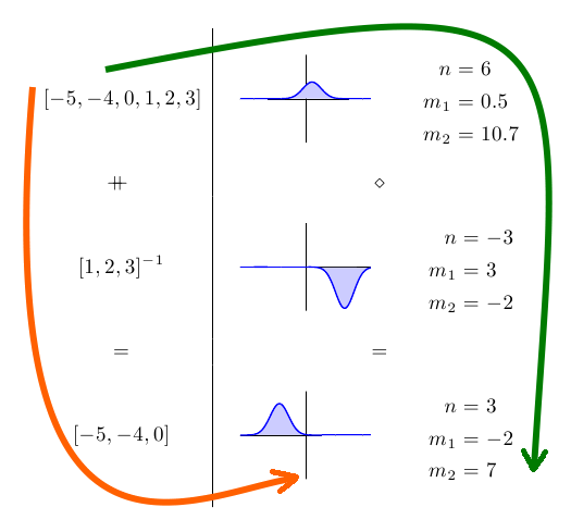
On the left hand side, we have some data sets, and on the right hand side, we have the corresponding Gaussian distributions and their parameters.  Because training the Gaussian is a homomorphism, it doesn’t matter whether we follow the orange or green paths to get to our final answer.  We get the exact same answer either way.

Based on this property alone, we get the three “free” properties I mentioned in the introduction.  (1) We get an online algorithm for free.  The function add1dp can be used to add a single new point to an existing Gaussian distribution.  Let’s say I forgot about one of the graduate students—I’m sure this would never happen in real life—I can add their salary like this:

> gradstudents_updated_gaussian = add1dp gradstudents_gaussian (10e3::Double)

This updated Gaussian is exactly what we would get if we had included the new data point in the original data set.

(2) We get a parallel algorithm.  We can use the higher order function parallel to parallelize any application of train.  For example,

> gradstudents_parallel_gaussian = (parallel train) gradstudents :: Gaussian Double

The function parallel automatically detects the number of processors your computer has and evenly distributes the work load over them.  As we’ll see in the performance section, this results in perfect parallelization of the training function.  Parallelization literally could not be any simpler!

(3) We get asymptotically faster cross-validation; but that’s not really applicable to a Gaussian distribution so we’ll ignore it here.

One last note about the HomTrainer class: we never actually have to define the train function for our learning algorithm explicitly.  All we have to do is define the semigroup operation, and the compiler will derive our training function for us!  We’ll save a discussion of why this homomorphism property gives us these results for another post.  Instead, we’ll just take a look at what the Gaussian distribution’s semigroup operation looks like.

The Semigroup operation

Our Gaussian data type is defined as:

data Gaussian datapoint = Gaussian
    { n  :: !Int         -- The number of samples trained on
    , m1 :: !datapoint   -- The mean (first moment) of the trained distribution
    , m2 :: !datapoint   -- The variance (second moment) times (n-1)
    , dc :: !Int         -- The number of "dummy points" that have been added
    }

In order to estimate a Gaussian from a sample, we must find the total number of samples (n), the mean (m1), and the variance (calculated from m2).  (We’ll explain what dc means a little later.)  Therefore, we must figure out an appropriate definition for our semigroup operation below:

(Gaussian na m1a m2a dca) <> (Gaussian nb m1b m2b dcb) = Gaussian n' m1' m2' dc'

First, we calculate the number of samples n’. The number of samples in the resulting distribution is simply the sum of the number of samples in both the input distributions:

Second, we calculate the new average m1′. We start with the definition that the final mean is:

Then we split the summation according to whether the input element was from the left Gaussian a or right Gaussian b, and substitute with the definition of the mean above:

Notice that this is simply the weighted average of the two means. This makes intuitive sense. But there is a slight problem with this definition: When implemented on a computer with floating point arithmetic, we will get infinity whenever n’ is 0.  We solve this problem by adding a “dummy” element into the Gaussian whenever n’ would be zero.  This increases n’ from 0 to 1, preventing the division by 0.  The variable dc counts how many dummy variables have been added, so that we can remove them before performing calculations (e.g. finding the pdf) that would be affected by an incorrect number of samples.

Finally, we must calculate the new m2′. We start with the definition that the variance times (n-1) is:

(Note that the second half of the equation is a property of variance, and its derivation can be found on wikipedia.)

Then, we do some algebra, split the summations according to which input Gaussian the data point came from, and resubstitute the definition of m2 to get:

Notice that this equation has no divisions in it.  This is why we are storing m2 as the variance times (n-1) rather than simply the variance.  Adding in the extra divisions causes training our Gaussian distribution to run about 4x slower.  I’d say haskell is getting pretty fast if the number of floating point divisions we perform is impacting our code’s performance that much!

Performance

This algebraic interpretation of the Gaussian distribution has excellent time and space performance.  To show this, we’ll compare performance to the excellent Haskell package called “statistics” that also has support for Gaussian distributions.  We use the criterion package to create three tests:

> size = 10^8
> main = defaultMain
>     [ bench "statistics-Gaussian" $ whnf (normalFromSample . VU.enumFromN 0) (size)
>     , bench "HLearn-Gaussian" $ whnf
>         (train :: VU.Vector Double -> Gaussian Double)
>         (VU.enumFromN (0::Double) size)
>     , bench "HLearn-Gaussian-Parallel" $ whnf
>         (parallel $ (train :: VU.Vector Double -> Gaussian Double))
>         (VU.enumFromN (0::Double) size)
>     ]

In these test, we time three different methods of constructing Gaussian distributions given 100,000,000 data points.  On my laptop with 2 cores, I get these results:

statistics-Gaussian	2.85 sec
HLearn-Gaussian	1.91 sec
HLearn-Gaussian-Parallel	0.96 sec

 

Pretty nice!  The algebraic method managed to outperform the traditional method for training a Gaussian by a handy margin.  Plus, our parallel algorithm runs exactly twice as fast on two processors.  Theoretically, this should scale to an arbitrary number of processors, but I don’t have a bigger machine to try it out on.

Another interesting advantage of the HLearn library is that we can trade off time and space performance by changing which data structures store our data set.  Specifically, we can use the same functions to train on a list or an unboxed vector.  We do this by using the ConstraintKinds package on hackage that extends the base type classes like Functor and Foldable to work on classes that require constraints.  Thus, we have a Functor instance of Vector.Unboxed. This is not possible without ConstraintKinds.

Using this benchmark code:

main = do
    print $ (train [0..fromIntegral size::Double] :: Gaussian Double)
    print $ (train (VU.enumFromN (0::Double) size) :: Gaussian Double)

We generate the following heap profile:

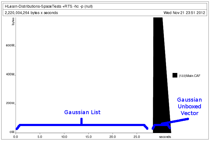
Processing the data as a vector requires that we allocate all the memory in advance.  This lets the program run faster, but prevents us from loading data sets larger than the amount of memory we have.  Processing the data as a list, however, allows us to allocate the memory only as we use it.  But because lists are boxed and lazy data structures, we must accept that our program will run about 10x slower.  Lucky for us, GHC takes care of all the boring details of making this happen seamlessly.  We only have to write our train function once.

Future Posts

There’s still at least four more major topics to cover in the HLearn library:  (1) We can extend this discussion to show how the Naive Bayes learning algorithm has a similar monoid and group structure.  (2) There are many more learning algorithms with group structures we can look into.  (3) We can look at exactly how all these higher order functions, like batch and parallel work under the hood.  And (4) we can see how the fast cross-validation I briefly mentioned works and why it’s important.

Subscribe to the RSS feed and stay tuned!