Introduction to data mining images
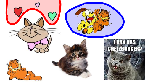
Image processing is one of those things people are still much better at than computers. Take this set of cats:

Just at a glance, you can easily tell the difference between the cartoon animals and the photographs. You can tell that the hearts in the top left probably don’t belong, and that Odie is tackling Garfield in the top right. The human brain does this really well on small datasets.
But what if we had thousands, millions, or even billions of images? Could we make an image search engine, where I give it a picture of an animal and it says what type it is? Could we make it automatically find patterns that people miss?
Yes! This post is the beginning of a series about how. Finding patterns in large databases of images is still an active research area, and these posts will hopefully make those results more accessible. The current research still isn’t perfect, but it’s probably much better than you’d guess.
The “black box” framework
There are three basic steps in data mining images:
STEP 1: Create the “black box”
STEP 2: Cluster
STEP 3: Run queries
That’s it!
… well … sort of …
There are many different algorithms that can be used at each step. Which ones you decide to use will depend on the type of information you’re mining from the images. The rest of this post gives a high level overview of how each of these steps works, and later posts will focus on specific implementations for each step.
STEP 1: Creating the black box
The black box defines the “distance” between two images. The smaller the distance, the more similar the images are. For example:
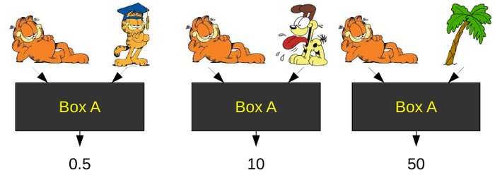 Garfield is very similar to himself, that’s why Box A gives him a low score–nearly zero. Odie is not very similar to Garfield, but he’s a lot closer than a palm tree. The specific numbers outputted don’t matter. All that matters is the ordering created by those numbers. In this case:
 Of course, if we compare against a different image, we will probably get a different ordering.
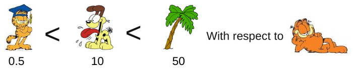
Likewise, we can get different orderings with a different black box. Let’s imagine that Box A was designed to determine if two pictures are of the same type of animal. If we test it on some new input, we might get:
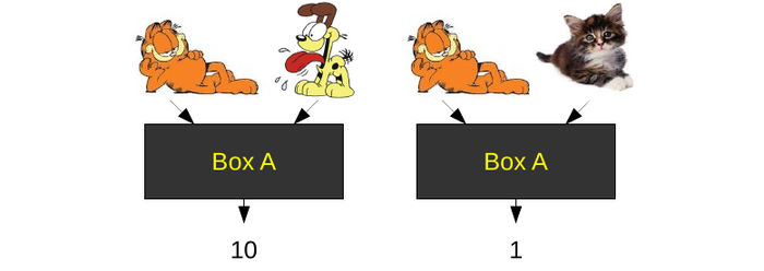 Notice that Box A thinks the real cat is more similar to Garfield than Odie is. Now let’s consider another black box. Imagine Box B is designed to see if two images were drawn in a similar style. Box B might give the following:
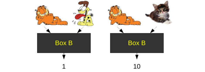
Box B gives the opposite results of box A.
Creating a good black box is the hardest part of data mining images. Most research is dedicated to this area, and most of this series will be focused on evaluating the performance of different black boxes. Which ones are good depends on your dataset and what information you’re trying to extract. Some general categories of black boxes we’ll look at are:
Histogram analysis (a simple technique that can be surprisingly effective on colored input)
Converting images into a time series (for analyzing the shapes of rigid objects, e.g. fruit)
Creating shock graphs (for analyzing the shapes of non-rigid objects, e.g. animals)
Komolgorov comlexity of the images (for comparing an image’s textures)
But first, let’s take a closer look at what makes a black box good.
Properties of a good black box
There are two more aspects of black boxes we must look at. First, every black box will be sensitive to certain features of an image and invariant to others. In the examples below, Box C is sensitive to shape, but invariant to color. Box D is sensitive to color, but invariant to shape.
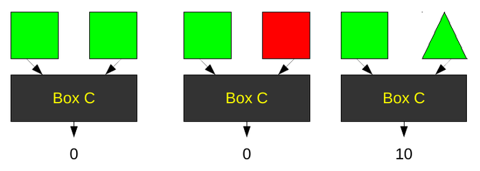
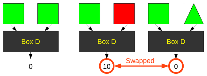
Most black box algorithms contain both sensitivities and invariances. These are the properties you will use to decide which black box is best for your application.
Second, a black box is a metric and as such must satisfy four criteria:
distance(x, y) ≥ 0 (non-negativity)
distance(x, y) = 0 if and only if x = y (identity of indiscernibles)
distance(x, y) = distance(y, x) (symmetry)
distance(x, z) ≤ distance(x, y) + distance(y, z) (subadditivity / triangle inequality).
If you don’t understand these criteria, don’t worry too much. All the black boxes we’ll look at in the rest of this series will satisfy these criteria automatically.
STEP 2: Cluster the images
Clustering is much easier than designing the black box. Clustering algorithms are used in many fields, so they have received much more attention. Some clustering algorithms commonly used are: K-means and Hierarchical clustering (i.e. Dendrograms).
There are many more as well. In general, you can use whatever clustering algorithm you want. When developing an application, most people will try several and pick whichever one happens to work the best for their data.
Here’s an example clustering of our cat data using Black Box A (i.e. by what the picture is of):
We’ve created three clusters. The red cluster contains hearts, the white cluster contains cats, and the blue cluster is an anomaly. It contains both a cat and a dog, and there is no easy way to separate them. If we had used a hierarchical classifier, the “contains cats and dogs cluster” might be a sub-cluster of the “contains cats cluster.”
Here’s the same data clustered using Black Box B (i.e. by how the picture is drawn):
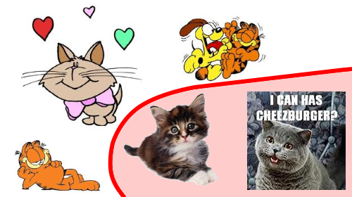
Now we have only two clusters: the white cluster contains cartoons, and the red cluster contains photographs.
One last note. Most of the CPU work gets done during this step. On large datasets, clustering can take hours to months depending on the algorithm and the speed of the black box. There are many tricks for speeding up clustering, which will take a look at in later posts.
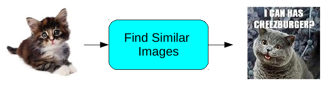
STEP 3: Run your query
Queries are fairly easy once the ground work is set up with the black box and clustering. Sometimes, all you want to know is how STEP 2 clustered your input. For example, you could query “how many types of animals are in this dataset?” The answer would just be the number of clusters using Box A. Typically, however, your query we will supply the database with an image and find similar images.
If we’ve done steps 1 and 2 well, this should take only seconds even when the database contains millions of images. Of course, it’s not always possible to do steps 1 and 2 well enough to make this happen. Later posts may cover some new techniques for speeding up the querying process.
The Rest of the Series
So far, we’ve seen that the black box framework for image datamining is very simple. The tricky part is putting the right algorithm in each step. In the rest of the series, we’ll look at a few different black boxes, and show how to efficiently combine them with a clustering algorithm. The different types of black boxes are the most interesting part of image mining, so we will focus on that first.