The categorical distribution's algebraic structure

The categorical distribution is the main distribution for handling discrete data. I like to think of it as a histogram. For example, let’s say Simon has a bag full of marbles. There are four “categories” of marbles—red, green, blue, and white. Now, if Simon reaches into the bag and randomly selects a marble, what’s the probability it will be green? We would use the categorical distribution to find out.
In this article, we’ll go over the math behind the categorical distribution, the algebraic structure of the distribution, and how to manipulate it within Haskell’s HLearn library. We’ll also see some examples of how this focus on algebra makes HLearn’s interface more powerful than other common statistical packages. Everything that we’re going to see is in a certain sense very “obvious” to a statistician, but this algebraic framework also makes it convenient. And since programmers are inherently lazy, this is a Very Good Thing.
Before delving into the “cool stuff,” we have to look at some of the mechanics of the HLearn library.
Preliminaries
The HLearn-distributions package contains all the functions we need to manipulate categorical distributions. Let’s install it:
$ cabal install HLearn-distributions-1.1We import our libraries:
>import Control.DeepSeq
>import HLearn.Algebra
>import HLearn.Models.Distributions
We create a data type for Simon’s marbles:
>data Marble = Red | Green | Blue | White
>    deriving (Read,Show,Eq,Ord)
The easiest way to represent Simon’s bag of marbles is with a list:
>simonBag :: [Marble]
>simonBag = [Red, Red, Red, Green, Blue, Green, Red, Blue, Green, Green, Red, Red, Blue, Red, Red, Red, White]
And now we’re ready to train a categorical distribution of the marbles in Simon’s bag:
>simonDist = train simonBag :: Categorical Double MarbleWe can load up ghci and plot the distribution with the conveniently named function plotDistribution:
ghci> plotDistribution (plotFile "simonDist" $ PDF 400 300) simonDistThis gives us a histogram of probabilities:
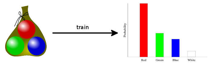
In the HLearn library, every statistical model is generated from data using either train or train’. Because these functions are overloaded, we must specify the type of simonDist so that the compiler knows which model to generate. Categorical takes two parameters. The first is the type of the discrete data (Marble). The second is the type of the probability (Double). We could easily create Categorical distributions with different types depending on the requirements for our application. For example:
>stringDist = train (map show simonBag) :: Categorical Float StringThis is the first “cool thing” about Categorical: We can make distributions over any user-defined type. This makes programming with probabilities easier, more intuitive, and more convenient. Most other statistical libraries would require you to assign numbers corresponding to each color of marble, and then create a distribution over those numbers.
Now that we have a distribution, we can find some probabilities. If Simon pulls a marble from the bag, what’s the probability that it would Red?
We can use the pdf function to do this calculation for us:
ghci> pdf simonDist Red
0.5294117647058824
ghci> pdf simonDist Blue
0.17647058823529413
ghci> pdf simonDist Green
0.23529411764705882
ghci> pdf simonDist White
0.058823529411764705
If we sum all the probabilities, as expected we would get 1:
ghci> sum $ map (pdf simonDist) [Red,Green,Blue,White]
1.0
Due to rounding errors, you may not always get 1. If you absolutely, positively, have to avoid rounding errors, you should use Rational probabilities:
>simonDistRational = train simonBag :: Categorical Rational MarbleRationals are slower, but won’t be subject to floating point errors.
This is just about all the functionality you would get in a “normal” stats package like R or NumPy. But using Haskell’s nice support for algebra, we can get some extra cool features.
Semigroup
First, let’s talk about semigroups. A semigroup is any data structure that has a binary operation (<>) that joins two of those data structures together. The categorical distribution is a semigroup.
Don wants to play marbles with Simon, and he has his own bag. Don’s bag contains only red and blue marbles:
>donBag = [Red,Blue,Red,Blue,Red,Blue,Blue,Red,Blue,Blue]We can train a categorical distribution on Don’s bag in the same way we did earlier:
>donDist = train donBag :: Categorical Double MarbleIn order to play marbles together, Don and Simon will have to add their bags together.
>bothBag = simonBag ++ donBagNow, we have two options for training our distribution. First is the naive way, we can train the distribution directly on the combined bag:
>bothDist = train bothBag :: Categorical Double MarbleThis is the way we would have to approach this problem in most statistical libraries. But with HLearn, we have a more efficient alternative. We can combine the trained distributions using the semigroup operation:
>bothDist' = simonDist <> donDistUnder the hood, the categorical distribution stores the number of times each possibility occurred in the training data. The <> operator just adds the corresponding counts from each distribution together:
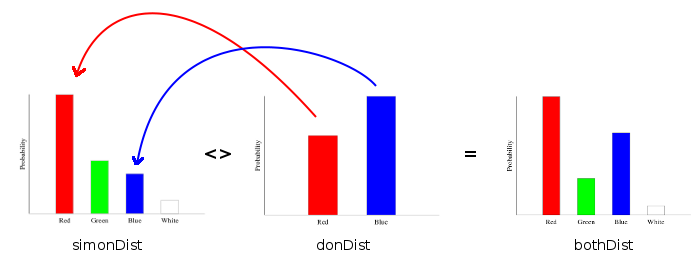
This method is more efficient because it avoids repeating work we’ve already done. Categorical’s semigroup operation runs in time O(1), so no matter how big the bags are, we can calculate the distribution very quickly. The naive method, in contrast, requires time O(n). If our bags had millions or billions of marbles inside them, this would be a considerable savings!
We get another cool performance trick “for free” based on the fact that Categorical is a semigroup: The function train can be automatically parallelized using the higher order function parallel. I won’t go into the details about how this works, but here’s how you do it in practice.
First, we must show the compiler how to resolve the Marble data type down to “normal form.” This basically means we must show the compiler how to fully compute the data type. (We only have to do this because Marble is a type we created. If we were using a built in type, like a String, we could skip this step.) This is fairly easy for a type as simple as Marble:
>instance NFData Marble where
>    rnf Red   = ()
>    rnf Blue  = ()
>    rnf Green = ()
>    rnf White = ()
Then, we can perform the parallel computation by:
>simonDist_par = parallel train simonBag :: Categorical Double MarbleOther languages require a programmer to manually create parallel versions of their functions. But in Haskell with the HLearn library, we get these parallel versions for free! All we have to do is ask for it!
Monoid
A monoid is a semigroup with an empty element, which is called mempty in Haskell. It obeys the law that:
M <> mempty == mempty <> M == MAnd it is easy to show that Categorical is also a monoid. We get this empty element by training on an empty data set:
mempty = train ([] :: [Marble]) :: Categorical Double MarbleThe HomTrainer type class requires that all its instances also be instances of Monoid. This lets the compiler automatically derive “online trainers” for us. An online trainer can add new data points to our statistical model without retraining it from scratch.
For example, we could use the function add1dp (stands for: add one data point) to add another white marble into Simon’s bag:
>simonDistWhite = add1dp simonDist WhiteThis also gives us another approach for our earlier problem of combining Simon and Don’s bags. We could use the function addBatch:
>bothDist'' = addBatch simonDist donBagBecause Categorical is a monoid, we maintain the property that:
bothDist == bothDist' == bothDist''Again, statisticians have always known that you could add new points into a categorical distribution without training from scratch. The cool thing here is that the compiler is deriving all of these functions for us, and it’s giving us a** consistent interface for use with different data structures. All we had to do to get these benefits was tell the compiler that Categorical is a monoid. This makes designing and programming libraries much easier, quicker, and less error prone**.
Group
A group is a monoid with the additional property that all elements have an inverse. This lets us perform subtraction on groups. And Categorical is a group.
Ed wants to play marbles too, but he doesn’t have any of his own. So Simon offers to give Ed some of from his own bag. He gives Ed one of each color:
>edBag = [Red,Green,Blue,White]Now, if Simon draws a marble from his bag, what’s the probability it will be blue?
To answer this question without algebra, we’d have to go back to the original data set, remove the marbles Simon gave Ed, then retrain the distribution. This is awkward and computationally expensive. But if we take advantage of Categorical’s group structure, we can just subtract directly from the distribution itself. This makes more sense intuitively and is easier computationally.
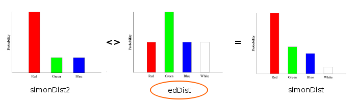
>simonDist2 = subBatch simonDist edBagThis is a shorthand notation for using the group operations directly:
>edDist = train edBag :: Categorical Double Marble
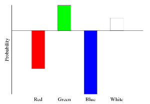
>simonDist2' = simonDist <> (inverse edDist)The way the inverse operation works is it multiplies the counts for each category by -1. In picture form, this flips the distribution upside down:
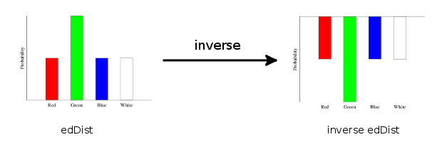
Then, adding an upside down distribution to a normal one is just subtracting the histogram columns and renormalizing:
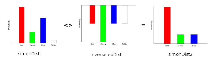
Notice that the green bar in edDist looks really big—much bigger than the green bar in simonDist. But when we subtract it away from simonDist, we still have some green marbles left over in simonDist2. This is because the histogram is only showing the probability of a green marble, and not the actual number of marbles.
Finally, there’s one more crazy trick we can perform with the Categorical group. It’s perfectly okay to have both positive and negative marbles in the same distribution. For example:
ghci> plotDistribution (plotFile "mixedDist" $ PDF 400 300) (edDist <> (inverse donDist))results in:
Most statisticians would probably say that these upside down Categoricals are not “real distributions.” But at the very least, they are a convenient mathematical trick that makes working with distributions much more pleasant.
Module
Finally, an R-Module is a group with two additional properties. First, it is abelian. That means <> is commutative. So, for all a, b:
a <> b == b <> aSecond, the data type supports multiplication by any element in the ring** R**. In Haskell, you can think of a ring as any member of the Num type class.
How is this useful? It let’s “retrain” our distribution on the data points it has already seen. Back to the example…
Well, Ed—being the clever guy that he is—recently developed a marble copying machine. That’s right! You just stick some marbles in on one end, and on the other end out pop 10 exact duplicates. Ed’s not just clever, but pretty nice too. He duplicates his new marbles and gives all of them back to Simon. What’s Simon’s new distribution look like?
Again, the naive way to answer this question would be to retrain from scratch:
>duplicateBag = simonBag ++ (concat $ replicate 10 edBag)
>duplicateDist = train duplicateBag :: Categorical Double Marble
Slightly better is to take advantage of the Semigroup property, and just apply that over and over again:
>duplicateDist' = simonDist2 <> (foldl1 (<>) $ replicate 10 edDist)But even better is to take advantage of the fact that Categorical is a module and the (.*) operator:
>duplicateDist'' = simonDist2 <> 10 .* edDistIn picture form:

Also notice that without the scalar multiplication, we would get back our original distribution:
Another way to think about the module’s scalar multiplication is that it allows us to weight our distributions.
Ed just realized that he still needs a marble, and has decided to take one. Someone has left their Marble bag sitting nearby, but he’s not sure whose it is. He thinks that Simon is more forgetful than Don is, so he assigns a 60% probability that the bag is Simon’s and a 40% probability that it is Don’s. When he takes a marble, what’s the probability that it is red?
We create a weighted distribution using module multiplication:
>weightedDist = 0.6 .* simonDist <> 0.4 .* donDistThen in ghci:
ghci> pdf weightedDist Red
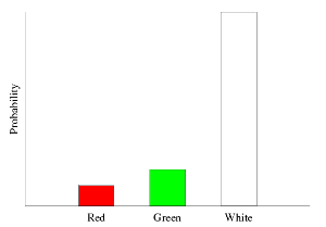
0.4929577464788732We can also train directly on weighted data using the trainW function:
>weightedDataDist = trainW [(0.4,Red),(0.5,Green),(0.2,Green),(3.7,White)] :: Categorical Double Marblewhich gives us:
The Takeaway and next posts
Talking about the categorical distribution in algebraic terms let’s us do some cool new stuff with our distributions that we can’t easily do in other libraries. None of this is statistically ground breaking. The cool thing is that algebra just makes everything so convenient to work with.
I think I’ll do another post on some cool tricks with the kernel density estimator that are not possible at all in other libraries, then do a post about the category (formal category-theoretic sense) of statistical training methods. At that point, we’ll be ready to jump into machine learning tasks. Depending on my mood we might take a pit stop to discuss the computational aspects of free groups and modules and how these relate to machine learning applications.