Using HMMs in Haskell for Bioinformatics

This is a tutorial for how to use Hidden Markov Models (HMMs) in Haskell. We will use the Data.HMM package to find genes in the second chromosome of Vitis vinifera: the wine grape vine. Predicting gene locations is a common task in bioinformatics that HMMs have proven good at.
The basic procedure has three steps. First, we create an HMM to model the chromosome. We do this by running the Baum-Welch training algorithm on all the DNA. Second, we create an HMM to model transcription factor binding sites. This is where genes are located. Finally, we use Viterbi’s algorithm to determine which HMM best models the DNA at a given location in the chromosome. If it’s the first, this is probably not the start of a gene. If it’s the second, then we’ve found a gene!
Unfortunately, it’s beyond the scope of this tutorial to go into the math of HMMs and how they work. Instead, we will focus on how to use them in practice. And like all good Haskell tutorials, this page is actually a literate Haskell program, so you can simply cut and paste it into your favorite text editor to run it.
The code
Before we do anything else, we must import the Data.HMM library, and some other libraries for the program
>import Data.HMM
>import Control.Monad
>import Data.Array
>import System.IO
Now, let’s create our first HMM. The HMM datatype is:
data HMM stateType eventType = HMM { states :: [stateType]
                                   , events :: [eventType]
                                   , initProbs :: (stateType -> Prob)
                                   , transMatrix :: (stateType -> stateType -> Prob)
                                   , outMatrix :: (stateType -> eventType -> Prob)
                                   }
Notice that states and events can be any type supported by Haskell. In this example, we will be using both integers and strings for the states, and characters for the events. DNA is composed of 4 base pairs that get repeated over and over: adenine (A), guanine (G), cytosine (C), and thymine (T), so “AGCT” will be the list of our events.
We’ll start by creating a simple HMM by hand:
>hmm1 = HMM { states=[1,2]
>           , events=['A','G','C','T']
>           , initProbs = ip
>           , transMatrix = tm
>           , outMatrix = om
>           }
>
>ip s
>    | s == 1  = 0.1
>    | s == 2  = 0.9
>
>tm s1 s2
>    | s1==1 && s2==1    = 0.9
>    | s1==1 && s2==2    = 0.1
>    | s1==2 && s2==1    = 0.5
>    | s1==2 && s2==2    = 0.5
>
>om s e
>    | s==1 && e=='A'    = 0.4
>    | s==1 && e=='G'    = 0.1
>    | s==1 && e=='C'    = 0.1
>    | s==1 && e=='T'    = 0.4
>    | s==2 && e=='A'    = 0.1
>    | s==2 && e=='G'    = 0.4
>    | s==2 && e=='C'    = 0.4
>    | s==2 && e=='T'    = 0.1
While creating HMMs manually is straightforward, we will typically want to start with one of the built in HMMs. This simplest way to do this is the function simpleHMM:
>hmm2 = simpleHMM [1,2] "AGCT"hmm2 is an HMM with the same states and events as hmm1, but all the initial, transition, and output probabilities are distributed in an unknown manner. This is okay, however, because we will normally want to train our HMM using Baum-Welch to determine those parameters automatically.
Another simple way to create an HMM is by creating a non-hidden Markov model with the simpleMM command. (Note the absence of an “H”) Below, hmm3 is a 3rd order Markov model for DNA:
>hmm3 = simpleMM "AGCT" 3Now, how do we train our model? The standard algorithm is called Baum-Welch. To illustrate the process, we’ll create a short array of DNA, then call three iterations of baumWelch on it.
>dnaArray = listArray (1,20) "AAAAGGGGCTCTCTCCAACC"
>hmm4 = baumWelch hmm3 dnaArray 3
We use arrays instead of lists because this gives us better performance when we start passing large training data to Baum-Welch. Doing three iterations is completely arbitrary. Baum-Welch is guaranteed to converge, but there is no way of knowing how long that will take.
Now, let’s train our HMM on an entire chromosome. We will use the winegrape-chromosome2 file. This DNA file was downloaded from the plant genomics database. We can load and process it like this:
>loadDNAArray len = do
>    let dnaArray = listArray (1,len) $ filter isBP dna
>    return dnaArray
>    where
>          isBP x = if x `elem` "AGCT" -- This filters out the "N" base pair
>                      then True       -- "N" means it could be any bp
>                      else False      -- so this should not affect results too much
>
>createDNAhmm file len hmm = do
>    let hmm' = baumWelch hmm dna 10
>    putStrLn $ show hmm'
>    saveHMM file hmm'
>    return hmm'
The loadDNAArray function simply loads the DNA from the file into an array, and the createDNAhmm function actually calls the Baum-Welch algorithm. This function can take a while on long inputs—and DNA is a long input!—so we also pass a file parameter for it to save our HMM when it’s done for later use. Now let’s create our HMM:
>hmmDNA = createDNAhmm "trainedDNA.hmm" 50000 hmm3This call takes almost a full day on my laptop. Luckily, you don’t have to repeat it. The Data.HMM.HMMFile module allows us to write our HMMs to disk and retrieve them later. Simply download trainedDNA.hmm and then call loadHMM:
>hmmDNA_file = loadHMM "trainedDNA.hmm" :: IO (HMM String Char)NOTE: Whenever you use loadHMM, you must specify the type of the resulting HMM. loadHMM relies on the built-in “read” function, and this cannot work unless you specify the type!
Great! Now, we have a fully trained HMM for our chromosome. Our next step is to train another HMM on the transcription factor binding sites. There are many advanced ways to do this (e.g. Profile HMMs), but that’s beyond the scope of this tutorial. We’re simply going to download a list of TF binding sites, concatenate them, then train our HMM on them. This won’t be as effective, but saves us from taking an unnecessary tangent.
>createTFhmm file hmm = do
>    x <- strTF
>    let hmm' = baumWelch hmm (listArray (1,length x) x) 10
>    putStrLn $ show hmm'
>    saveHMM file hmm'
>    return hmm'
>    where
>          strTF = liftM (concat . map ( (++) "") ) loadTF
>          loadTF = liftM (filter isValidTF) $ (liftM lines) $ readFile "TFBindingSites"
>          isValidTF str = (length str > 0) && (not $ elemChecker "#(/)[]|N" str)
>
>elemChecker :: (Eq a) => [a] -> [a] -> Bool
>elemChecker elemList list
>    | elemList == []  = False
>    | otherwise       = if (head elemList) `elem` list
>                           then True
>                           else elemChecker (tail elemList) list
Now, let’s create our transcription factor HMM:
>hmmTF = createTFhmm "trainedTF.hmm" $ simpleMM "AGCT" 3Or if you’re in a hurry, just download trainedTF.hmm and load it:
>hmmTF_file = loadHMM "trainedTF.hmm" :: IO (HMM String Char)So now we have 2 HMMs, how are we going to use them? We’ll combine the two HMMs into a single HMM, then use Viterbi’s algorithm to determine which HMM best characterizes our DNA at a given point. If it’s hmmDNA, then we do not have a TF binding site at that location, but if it’s hmmTF, then we probably do.
The Data.HMM library provides another convenient function for combining HMMs, hmmJoin. It adds transitions from every state in the first HMM to every state in the second, and vice versa, using the “joinParam” to determine the relative probability of making that transition. This is the simplest way to combine to HMMs. If you want more control over how they get combined, you can implement your own version.
>findGenes len joinParam hout = do
>    hmmTF <- loadHMM "hmm/TF-3.hmm" :: IO (HMM String Char)
>    hmmDNA <- loadHMM "hmm/autowinegrape-1000-3.hmm"  :: IO (HMM String Char)
>    let hmm' = seq hmmDNA $ seq hmmTF $ hmmJoin hmmTF hmmDNA joinParam
>    dna <- loadDNAArray len
>    hPutStrLn hout ("len="++show len++",joinParam="++show joinParam++" -> "++(show $ concat $ map (show . fst) $ viterbi hmm' dna))
>
>main = do
>    hout     mapM_ (\len -> mapM_ (\jp -> findGenes len jp hout) [0.5,0.51,0.52,0.53,0.54,0.55,0.56,0.57,0.58,0.59,0.6]) [50000]
>    hClose hout
Finally, our main function runs findGenes with several different joinParams. These act as thresholds for finding where the genes actually occur. You can download the full results here.
How should we interpret these results? Let’s look at the output from around 38000 base pairs into the chromosome:
jP=0.50 -> 222222222222222222222222222222222222222222222222222222
jP=0.51 -> 222222222222222222222222222222222222222222222222222222
jP=0.52 -> 222222222222222222222222222222222222222222222222222222
jP=0.53 -> 222222222222222222222222222222222222222222222222222222
jP=0.54 -> 222222222222222222222222222222222222222222222222222222
jP=0.55 -> 222222222222222222222222222222222222222222222222222222
jP=0.56 -> 222222222222222222222222222211112222222222222222222222
jP=0.57 -> 222222222222222222222222222211112222222222222111222222
jP=0.58 -> 222221111111112222222222222211111122222222222111222222
jP=0.59 -> 222221111111112222211111111111111122211111111111222222
jP=0.60 -> 222221111111112222211111111111111111111111111111112222
Everywhere where there is a 2, Viterbi selected hmmDNA; where there is a 1, Viterbi selected the hmmTF. Whether you select this area as a likely candidate for a transcription factor binding site depends on how you set your join parameter.
Now that you’re familiar with how the Data.HMM module works, let’s look at its performance characteristics.
Performance
Overall, the Data.HMM package performs well on medium size datasets of up to about 10,000 items. Unfortunately, on larger datasets, performance begins to suffer. Algorithms that should be running in linear time start taking super-linear time, presumably because Haskell’s garbage collector is interfering. More work is needed to determine the exact cause and fix it. Still, performance remains tractable on these large datasets up to 100,000 items, which is the largest I tried.
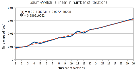
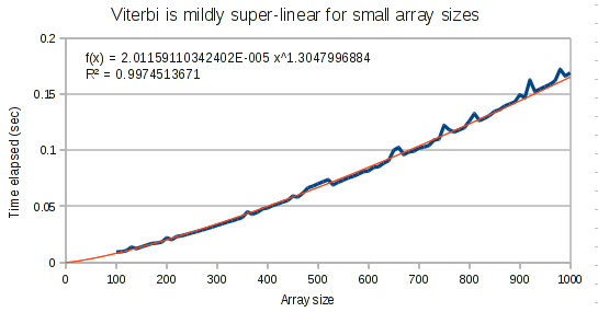
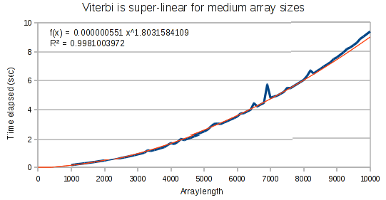
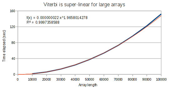
I ran these tests using haskell’s Data.Criterion package. Criterion conveniently allows you to define multiple tests and does all the statistical analysis of them. For these tests, I did 3 trials each, and ran them on my Core 2 duo laptop. The code for the tests can be found in the HMMPerf.hs file. In all graphs, the blue line is actual performance data and the red line is a best fit curve.
Baum-Welch’s performance
First, as expected we find that Baum-Welch runs in linear time based on the number of iterations. In an imperative language, there would be no point in even testing this. But in Haskell, laziness can rear its head in unexpected ways, so it is important to ensure this is linear.
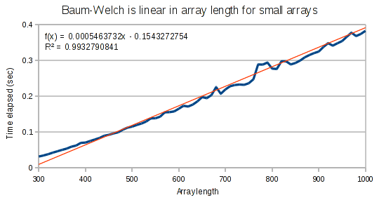
For small arrays, Baum-Welch runs in linear time.
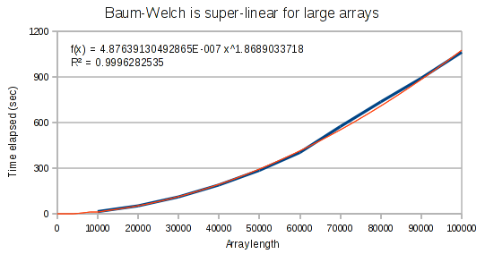
But for larger arrays, it runs in super-linear time. It is interesting that the exponent on our polynomial function is not quite at 2. This provides evidence that the performance hit has to do with the Haskell compiler and not an incorrect implementation.
Viterbi’s performance
As expected, the Viterbi runs in quadratic time on the number of states in the HMM.
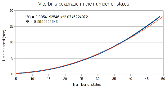
The curves for the Viterbi algorithm clearly demonstrate that something weird is going on. At small array sizes, Viterbi is only mildly super-linear. It’s best fit polynomial curve has an exponent of only 1.3. But at medium array lengths, this exponent increases to 1.8, and at large array lengths, the exponent increases to 1.97.
Conclusion
Data.HMM is a great tool if you just need a small HMM in your Haskell application for some reason. If you’re going to be making heavy use of HMMs and don’t specifically need to interact with Haskell, it’s probably better to use a package written in C++ that’s been optimized for speed.